Metagenomics + Microbial Surveillance Virtual Training Project
MILRD
Important Announcement 1
Before we start, everyone must complete the Pre-VTP survey: https://forms.gle/FA3gmijzCVf6Kiuv8
If you haven’t done this, please take 5 minutes to complete this now.
Important Announcement 2
Here is a Google Sheet that contains Sample Assignments, AWS and R addresses/info, and Participant Info:
https://docs.google.com/spreadsheets/d/1kGShY2587v0tYbqlc2G3v_vh6D5Ynu3fpEY_izYQzYY/edit?usp=sharing
Overview
Introduction to the project.
Rationale for the MetaSub Project
Overview: bioinformatics analyses you’ll perform
1. Introduction to the project.
The primary goal of this project is to use the Linux and R programming languages to bioinformatically characterize, quantify and visualize the species composition of urban microbiome samples (i.e. subway swabs) from raw data to completed analysis.
What is bioinformatics?
Think, Room (4-5 ppl), Share:
1-minute: think about one lab, activity, or lesson you prevously taught that had an element that could have been explored using bioinformatics analysis? (Explain)
3-minutes: divide into breakout rooms and discuss with your group
2-minutes: re-join the main meeting room and present 1-2 examples to the other participants.
Why is the metagenomics application of bioinformatics useful?
In case you (or more likely, your students) are thinking, “How would someone be able to use this knowledge in real life?”, here are three real-world applications of the metagenomics analysis technique you will learn:
Research Applications: you can ask questions about the similarity of microbiome samples, the prevalence/emergence of antimicrobial resistant strains, etc. The Metasub Project, which is where the data you’ll analyze in this VTP comes from, would be an example of this application.Clinical Applications: This technique is already being employed by some biotech startups, like Karius (https://kariusdx.com/), to rapidly diagnose blood-borne infections.Biotech/Industry Applications: Some companies offer microbial surveillance services to identify and monitor the presence of resistant pathogens (e.g. on hospital surfaces). One such startup called Biotia (https://www.biotia.io/) was spun out of the Mason lab (the same Cornell Med lab that created the Metasub project) and utilizes many of the same techniques that you will employ in this VTP.”
In a broader sense, bioinformatics is a subdivision of data science; principles learned in the former are highly relevant to the latter. We’ll point these out as we go along.
History of metagenomics:
Example: Clinical Application of Metagenomics:
Think, Room (4-5 ppl), Share:
1-minute: Come up with one potential application of metagenomics not discussed here.
3-minutes: divide into breakout rooms and discuss with your group
2-minutes: re-join the main meeting room and present 1-2 examples from your breakout room to the other participants.
2. Rationale for the MetaSub Project
To accomplish this goals in this project, we will use data from the Metasub project, an effort to characterize the “built environment” microbiomes of mass transit systems around the world, headed by Dr. Chris Mason’s lab at Weill Cornell Medical Center (http://www.masonlab.net/).
Here’s the recent Metasub paper in case you haven’t seen it and would like to review it later: https://milrd.org/wp-content/uploads/2022/09/Cell_A-global-metagenomic-map-of-urban-microbiomesand-antimicrobial-resistance.pdf
(To be frank, this article is a bit challenging to read, so we suggest you review it later on if you’re inclined, after you’ve done a bit of the project.)
Some additional information in case you’re interested:
New York Times article about the Metasub Project: https://www.nytimes.com/2021/05/26/science/microbes-subway-metasub-mason.html?smid=url-share
Metasub Project website: http://metasub.org
Metasub was borne out of a project called PathoMap (also from the Mason lab), which began in summer 2013 to profile the New York City metagenome in, around, and below NYC on mass-transit areas of the built environment, focusing on the subway.
Here’s the Pathomap paper in case you would like to review it later: https://milrd.org/wp-content/uploads/2022/09/Geospatial-Resolution-of-Human-and-Bacterial-Diversity-with-City-Scale-Metagenomics.pdf
Pathomap sought to establish baseline profiles across the subway system, identify potential bio-threats, and provide an additional level of data that can be used by the city to create a “smart city;” i.e., one that uses high- dimensional data to improve city planning, management, and human health.”
Metasub extended the Pathomap project based on the recognition that NYC is not the only city in the world that could benefit from a systematic, longitudinal metagenomic profile of its subway system.
Although NYC subway has the most stations, it ranks 7th in the world in term of the number of riders per year. A wide variety of population density, length, and climate types define the busiest subways of the world, ranging from cold (Moscow) to temperate (New York City, Paris), to subtropical (Mexico City) and tropical (São Paulo).
To address this gap in our knowledge of the built environment, the Mason lab created Metasub: an international consortium of laboratories to establish a world-wide “DNA map” of microbiomes in mass transit systems.
Take a look at Figure 1, which provides an overview of the Pathomap project’s design and execution:

As you can see, the researchers collected samples from
New York City’s five boroughs
Collected samples from the 466 subway stations of NYC across the 24 subway lines
extracted, sequenced, QC’d and analyzed DNA
Mapped the distribution of taxa identified from the entire pooled dataset, and
presented geospatial analysis of a highly prominent genus, Pseudomonas
Notably, as seen in (D), nearly half of the DNA sequenced (48%) did not match any known organism, underscoring the vast wealth of likely unknown organisms that surround passengers every day.
Think, Room (4-5 ppl), Share:
1-minute: Why do you think so much of the sequenced DNA did not match any known organism?
3-minutes: divide into breakout rooms and discuss with your group
2-minutes: re-join the main meeting room and present 1-2 examples from your breakout room to the other participants.
Now, let’s focus on Fig 1C, as samples from the Metasub project were collected, sequenced, and analyzed in a similar manner to the Pathomap project. Here’s a simplified version of what the Mason lab did in Fig 1C:

3. Overview: bioinformatics analyses you’ll perform
This guide is intended to teach you how to teach you one component of metagenomic analysis: how to plot abundances at the “phylum” level for each metagenomics sample.
Throughout the VTP, each participant characterizes, quantifies and visualize microbial metagenomics data from sequenced swabs of public urban environments on their own AWS High Performance Compute instance. In the Linux terminal, they perform genomic data quality control, genome alignment, taxonomic characterization & abundance quantification, and in R, they viaualize results, conduct a principal component analysis. To conclude, they investigate their most abundant species and use the Patric database to consider how they would determine the strains of these species.
Linux Steps R Steps Subset Component
Think, Room (4-5 ppl), Share:
1-minute: Note that we’re using two programming languages (Linux/Bash and R). Why do you think it’s necessary to use two programming languages, and not just one?
3-minutes: divide into breakout rooms and discuss with your group
2-minutes: re-join the main meeting room and present 1-2 examples from your breakout room to the other participants.
All bioinformatics tasks will be performed in “the cloud” on an Amazon Web Services (AWS) hosted high performance compute instance.
What is cloud computing:
Think, Room (4-5 ppl), Share:
1-minute: Why do we (as well as professional researchers, data scientists, bioinformaticians) often need to perform analyses on the cloud?
3-minutes: divide into breakout rooms and discuss with your group
2-minutes: re-join the main meeting room and present 1-2 examples from your breakout room to the other participants.
What is R and RStusio
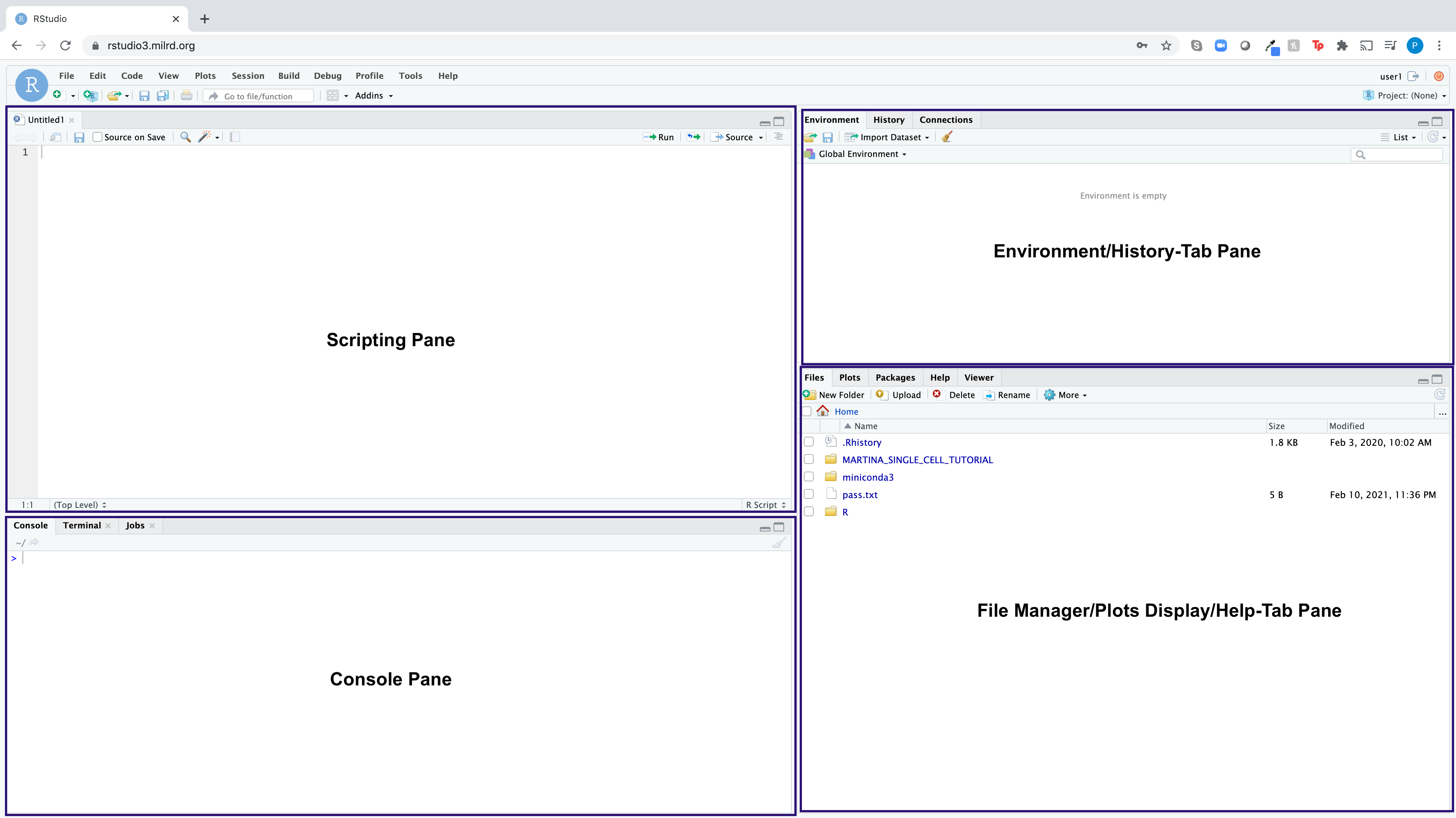
RStudio is an integrated development environment (IDE) for the open-source R programming language, which basically means it brings the core components of R (Scripting Pane, Console, Environment Pane, File Manager/Plots/Help Pane) into a quadrant-based user interface for efficient use.
Here is what the R dashboard looks like:

In R, code is always executed via the Console, but you have the
choice whether to execute that code in a Script (opened in the Scripting
Pane) or directly in the Console. Unless you need to quicly execute a
one-liner (e.g. setting a working directory using the setwd
command), you’ll want to be writing your code in a script, highlighting
it, and clicking Run to execute it in the console. This is
because you can easily edit code in a script and re-run it. Once code is
run in the Console it is not editable.
(1) Login to your AWS-hosted RStudio Instance (URL/username in the Google Sheet)
You are provided an instance of the R editor RStudio on AWS already waiting for you to use. Login to your AWS-hosted RStudio instance using the URL, username, and password assigned to you in the Google Sheet.
Please make sure the RStudio user interface dashboard looks as follows: Console Pane (Lower Left Quadrant), Scripting Pane (Upper Left Quadrant), File Manager/Plots Display/Help-Tab Pane (Lower Right Quadrant), Environment/History-Tab Pane (Upper Right Quadrant).
(2) Generate barplot(s) using subset of metagenomic samples
In this section, you will learn how to use R to generate two plots that help visualize the similarities and differences between a subset of the Metasub samples and compare it to metagenomics samples from the Human Microbiome project.
We have provided a subset of of metagnomics data
(taxa_table.csv) and one with, for your convenience. This
file contains taxonomically characterized and quantified metagenomics
data from nine microbiome samples: three from the human microbiome
project, three from the Metasub project, and three from a mystery
source.
First we will plot our samples as a stacked-barplot at the phylum level. A stacked-barplot shows a set of numbers as a series of columns one on top of each other colored by a label. In our case, a taxonomic profile is a set of numerical abundances labeled by the microbial species it belongs to.
Here’s how we make this plot in R:
library(ggplot2)   # These lines load additional libraries into our environment

taxa = read.csv('taxa_table.csv', header=TRUE, sep=',')  # Read our taxonomic table into a computational object from a file

taxa = taxa[taxa$rank == 'phylum',]  # This filters our taxonomic table to a specific taxonomic rank. One of Kingdom, Phylum, Class, Order, Family, Genus, Species. Play around with a few other ranks.

ggplot(taxa, aes(x=sample, y=percent_abundance, fill=taxon)) + # this creates a ggplot object. Can you figure out what the aes(...) section is doing?
  geom_bar(stat="identity") +  # this tells ggplot how we want our data to be displayed
  xlab('Sample') +  # These lines tell ggplot what our axis labels should be
  ylab('Abundance') +
  labs(fill='Phylum') +
theme(axis.text.x = element_text(angle = 90)) # this rotates the x-axis text 90 degrees(4) Generate barplot at the family level
- Modify code: edit your script to generate a barplot at the “family” level, by modifying this line of code:
taxa = taxa[taxa$rank == 'phylum',] Checkpoint (CP) 1 Please upload the
following to the Google Sheet:
Barplot at the phylum level. (To download this plot as a file, click the (+) Zoom button, right click on the plot and select “Save Image As”.)
Upload barplot at the family level. (To download this plot as a file, click the (+) Zoom button, right click on the plot and select “Save Image As”.)
Answer to these questions:
- Which line of code ingests data from the
taxa_table.csvfile into thetaxaobject (copy paste the exact line of code)?
- Which line of code ingests data from the
- Which line of code allows you to filter down to a specific taxonomic level?
- What is the
$operator doing in this line of code:taxa = taxa[taxa$rank == 'phylum',]?
- What is the
- Why wouldn’t you want to plot a barplot at the species level? (If you’re not sure, try it!)
- What can the barplots tell you about the similarities and dissimilarities of microbiome samples?
- What questions do barlots leave unanswered about microbiome samples?
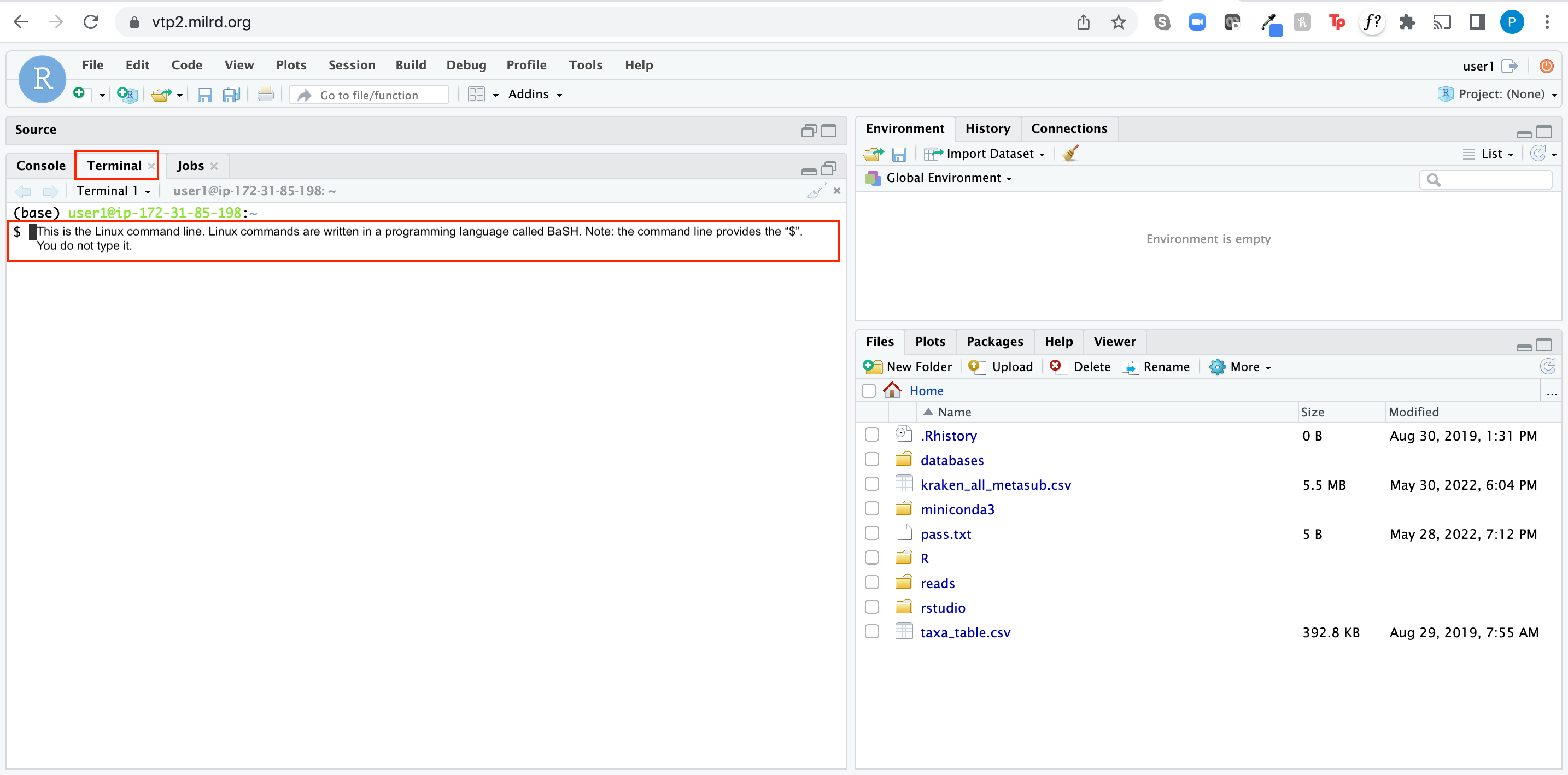
(5) Access your Linux terminal via your AWS-hosted RStudio instance
Access your Linux terminal by logging into RStudio via the web browser (can be found in the the Google Sheet.
Setup to your Linux environment:
It should look like this once you’re finished setting up your Linux environment:

(7) Look at your assigned dataset (time estimate: 10 min)
To make sure you undertstand the workflow, we’d like to first have
you complete the analysis with a small dataset. We’ve taken 50,000 reads
from the read1 and read2 files of each assigned sample. They are labeled
with the prefix mini_ and located in the reads
directory (files without the prefix mini are the original,
full-size files, which each contain millions of reads.)
Data from each Metasub sample is contained in two files—read1
(i.e. R1) and read2 (i.e.R2). This is because
the researchers paired-end sequenced each sample. When samples
are sequenced on an Illumina genomic sequencer researchers get to
decide: (1) the number of reads to generate for each sample library; (2)
the read length (within a range of ~50 - ~300 nucleotides); and (3)
whether to generate a single read or a pair of reads from each sequenced
DNA library fragment.
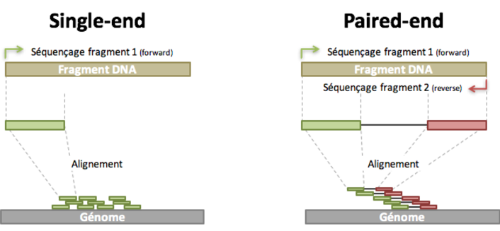
Here is an diagram that summarizes paired-end versus single-end sequencing:

A FASTQ record has the following format:
- A line starting with @, containing the sequence ID.
- One or more lines that contain the sequence.
- A new line starting with the character +, and being either empty or repeating the sequence ID.
- One or more lines that contain the quality scores.
Here’s an example of a FASTQ file with two records:
@071112_SLXA-EAS1_s_7:5:1:817:345
GGGTGATGGCCGCTGCCGATGGCGTCAAATCCCACC
+
IIIIIIIIIIIIIIIIIIIIIIIIIIIIII9IG9IC
@071112_SLXA-EAS1_s_7:5:1:801:338
GTTCAGGGATACGACGTTTGTATTTTAAGAATCTGA
+
IIIIIIIIIIIIIIIIIIIIIIIIIIIIIIII6IBI
Navigate to the reads directory (which contains the
“mini” fastq data):
$ cd ~/reads/PLEASE NOTE: make sure to complete all steps in this section from the
reads directory.
Take a look at the first 10 lines of your assigned fastq files:
$ zcat mini_my_reads.R1.fastq.gz | head

$ zcat mini_my_reads.R2.fastq.gz | head
(Please note: mini_my_reads is a placeholder for your
assigned miniature reads dataset.)
Checkpoint (CP) 3
In the Google Sheet, please:
Upload a screenshot of your zcat results.
Answer these questions:
- How are fastq files are structured? (i.e. What does line 1, line 2, line 3, and line 4, of each read signify?)
- Why are there two reads files for each sample?
(8) Remove adapters and filter-out low quality reads
Check AdapterRemoval is working by opening your terminal
and typing:
$ AdapterRemoval -h
You should see a long list of all the arguments that can be given to this tool.
Run AdapterRemoval on your mini sample (executable version):
$ AdapterRemoval --file1 mini_my_reads.R1.fastq.gz --file2 mini_my_reads.R2.fastq.gz --trimns --trimqualities --minquality 40 --threads 2 --gzip --output1 clean.mini_my_reads.R1.fastq.gz --output2 clean.mini_my_reads.R2.fastq.gzPlease note: mini_my_reads is a placeholder for your
assigned sample ID. The file extension .fq is a widely used
abbreviation for .fastq.
Run AdapterRemoval on your sample (explanatory version):
$ AdapterRemoval
--file1 mini_my_reads.R1.fastq.gz --file2 mini_my_reads.R2.fastq.gz
--trimns
--trimqualities --minquality 40
--threads 2
--gzip
--output1 clean.mini_my_reads.R1.fastq.gz --output2 clean.mini_my_reads.R2.fastq.gz - Calls the program you want to invoke.
- this tells the program where to find our input data.
- this tells the program to remove reads with ambiguous bases or ’N’s
- this tells the program to remove reads with low-quality bases
- this tells the computer to multithread the program with 2 cores
- this tells the program that both the input and output files are compressed with a program call gzip
- this tells the program where to put its output
Now we have read files that are clean. Look at one of the output files by running:
$ zcat clean.mini_my_reads.R1.fastq.gz | head

$ zcat clean.mini_my_reads.R2.fastq.gz | head
For comparison, look again at the first 10 lines of your raw reads:
$ zcat mini_my_reads.R1.fastq.gz | head

$ zcat mini_my_reads.R2.fastq.gz | head
Notice any differences between the Clean and Raw reads? If so, write them down.
Count the number of reads in each of your cleaned fastq files by running:
$ zcat clean.mini_reads.R1.fastq.gz | wc -l and manually
dividing by four.
$ zcat clean.mini_reads.R2.fastq.gz | wc -l and manually
dividing by four.
Count the number of reads in each of your raw (i.e. initial) fastq files by running:
$ zcat mini_reads.R1.fastq.gz | wc -l and manually
dividing by four.
$ zcat mini_reads.R2.fastq.gz | wc -l and manually
dividing by four.
CP 4 In the Google Sheet, please: 1.
Upload a screenshot of your zcat results. 2. Answer these questions:
- Do you notice any differences in the read lengths between your Raw and Cleaned reads? If so, what?
- Report the numbers of your Raw and Cleaned reads.
(9) Not shown: Remove contaminating human DNA from your sample
Researchers often decide at this point to remove DNA from unwanted species, such as human. DNA that we don’t want is called “Contaminating DNA”. We are not going to perform this step due to time constraints.
(10) Execute Metagenomic Analysis
Launch Kraken (executable version):
$ conda install --channel bioconda --yes kraken Launch Kraken (explanatory version):
$ conda  # the name of the package manager
install  # this is a subcommand, miniconda has several other functions
--channel bioconda
--yes  # give conda permission to install software
kraken  # the name of the program we are installing
You should now be able to test Kraken by running:
$ kraken --helpIf everything is working, we can now perform taxonomic classification on our data using this command (executable version):
$ kraken --gzip-compressed --fastq-input --threads 2 --paired --preload --db ~/databases/minikraken_20171101_8GB_dustmasked clean.mini_my_reads.R1.fastq.gz clean.mini_my_reads.R2.fastq.gz > mini_my_reads_taxonomic_report.csvBE SURE to replace mysampleID with your assigned sample
ID.
$ kraken --gzip-compressed --fastq-input --threads 2 --paired --preload --db ~/databases/minikraken_20171101_8GB_dustmasked clean.mini_my_reads.R1.fastq.gz clean.mini_my_reads.R2.fastq.gz > mini_my_reads_taxonomic_report.csvBE SURE to replace mysampleID with your assigned sample
ID.
If everything is working, we can now perform taxonomic classification on our data using this command (explanatory version):
$ kraken
--gzip-compressed  # tells kraken that our reads are compressed
--fastq-input  # tells kraken that our reads are formatted as fastq files
--threads 2  # uses 2 threads
--paired  # tells kraken that we have paired end data
--preload  # loads the database into RAM before running
--db ~/databases/minikraken_20171101_8GB_dustmasked  # tells kraken where to find the database
clean.mini_my_reads.R1.fastq.gz # Filepath to Read1 file
clean.mini_my_reads.R2.fastq.gz # Filepath to Read2 file
> mini_my_reads_taxonomic_report.csv
Once this command runs, take a look at the output by running:
$ head mini_my_reads_taxonomic_report.csv (the
head command prints the first 10 lines of any file to the
terminal)

Note Column 1 indicates whether it was classified by Kraken or not. Column 2 denotes the Read ID (line 1 of the fastq read record). Subsequent columns indicated taxonomic mappings, if any.
The mini_my_reads_taxonomic_report.csv is formatted for
storage efficiency and is not very useful for biological interpretation.
Convert this file to an .mpa format so that it can be
interpreted more easily:
$ kraken-mpa-report --db ~/databases/minikraken_20171101_8GB_dustmasked mini_my_reads_taxonomic_report.csv > mini_my_reads_final_taxonomic_results.mpaLook at the first 20 lines by executing:
$ head -20 mini_my_reads_final_taxonomic_results.mpaLook at the last 20 lines by executing:
$ tail -20 mini_my_reads_final_taxonomic_results.mpaPull out the species level assignments in your .mpa file
and store them in a .tsv file:
$ grep 's__' mini_my_reads_final_taxonomic_results.mpa > mini_my_reads_species_only.tsvLook at the first 10 lines:
$ head mini_my_reads_species_only.tsvSee how many species were identified:
$ wc -l mini_my_reads_species_only.tsvCP 5
In the Google Sheet, please:
Upload a screenshot of your
krakencommand output. (i.e. the one that states the % sequences classified and unclassified)Upload a screenshot of your
head -20 mini_my_reads_final_taxonomic_results.mpacommand.Upload a screenshot of your
tail -20 mini_my_reads_final_taxonomic_results.mpacommand.Answer these questions:
- What do d, p, and other abbreviations stand for?
- What do you the numbers at the end of each line signify?
- Why do you think Kraken can’t characterize some reads at all?
- Why do you think Kraken can’t characterize some reads down to the species level?
- When identifying only the species-level taxonomic assignments, what “search term” do you use in your code?
(11) Generate barplot using all kraken samples that you and your classmates analyzed
Now create a barplot with all of the metasub samples:
library(ggplot2)

taxa_all_barplot = read.csv('kraken_all_metasub.csv', header=TRUE, sep=',')

taxa_all_barplot = taxa_all_barplot[taxa_all_barplot$rank == 'phylum',]

taxa_all_barplot = taxa_all_barplot[taxa_all_barplot$percent_abundance >= 2,]

ggplot(taxa_all_barplot, aes(x=sample, y=percent_abundance, fill=taxon)) +

  geom_bar(stat="identity") +
  xlab('Sample') +
  ylab('Abundance') +
  labs(fill='Phylum') +
  theme(axis.text.x = element_text(angle = 90))
CP 6
Please upload the following to the Google Sheet:
- Barplot at the phylum level for all samples. (To download this plot as a file, click the (+) Zoom button, right click on the plot and select “Save Image As”.)
(12) Sort species abundance from highest to lowest
Read-in all of the Kraken data from the samples you and the other participants analyzed:
# Read-in all metasub data
taxa_all = read.csv('kraken_all_metasub.csv', header=TRUE, sep=',')

# Filter down to species level
taxa_all_spp = taxa_all[taxa_all$rank == 'species',]

# Sort to your sample. Be sure to specify your SampleID (e.g. SL342389) where indicated.
taxa_all_spp_mySampleID = taxa_all_spp[taxa_all_spp$sample == 'SampleID',]

# Order object from highest-to-lowest percent abundance
taxa_all_spp_mySampleID_ordered <- taxa_all_spp_mySampleID[order(taxa_all_spp_mySampleID$percent_abundance, decreasing = TRUE), ]

# Print top 5 most abundant species in your sample to the Console
head(taxa_all_spp_mySampleID_ordered, 5)
For your information, you can open
taxa_all_spp_mySampleID as a table in the Scripting Pane by
clicking on the name of the object in the Environment Pane. You can
order rows based on the incresing and decreasing values of a specific
column by clicking the ▲ and ▼ arrows of that column.
CP 7
In the Google Sheet:
- List the top 5 most abundant species in your sample.
(13) ID Potential Antibiotic Resistance Loci in the SPP in Your Assigned Sample
Navigate to the Bacterial and Viral Bioinformatics Resource Center (BV-BRC): https://www.bv-brc.org/
Use the tools in BV-BRC to ID at least one AMR locus/gene for the top 5 most abundant species in your sample.
- Select Taxa option from the “All Data Types” dropdown menu
- Search for a given species via the search bar
- Select the “species” result (usually the first one) by checking the box next to that row
- Click
TAXON OVERVIEWfrom the green column - Click the
Specialty Genestab - Click the blue
Filterbutton - For Property, select
Antibiotic Resitance - For Source, select PATRIC
- For Classification, search for
efflux pump conferring antibiotic resistanceusing the magnifying glass feature - Select a few of the results rows by checking their boxes
- Click the
FASTAoption in the green column and selectView FASTA DNAThis will show you the nucleotide sequences of the selected resistance loci.
Here’s a screencast using the species Staphylococcus aureus (Methicillin-resistant Staphylococcus aureus (MRSA) is a widely known antibiotic resistant hospital acquired infection):
CP 8
In the Google Sheet:
- List three
efflux pump conferring antibiotic resistancelocus IDs for the species you queried using the BV-BRC. - Hypothesize how you would figure out if a resistant strain of one of the abundant species in your sample was present.
4. Biology + Data Science in the Classroom
While the linux steps can be challenging to perform on a local computuer, students should be able to perform all R/RStudio related steps.
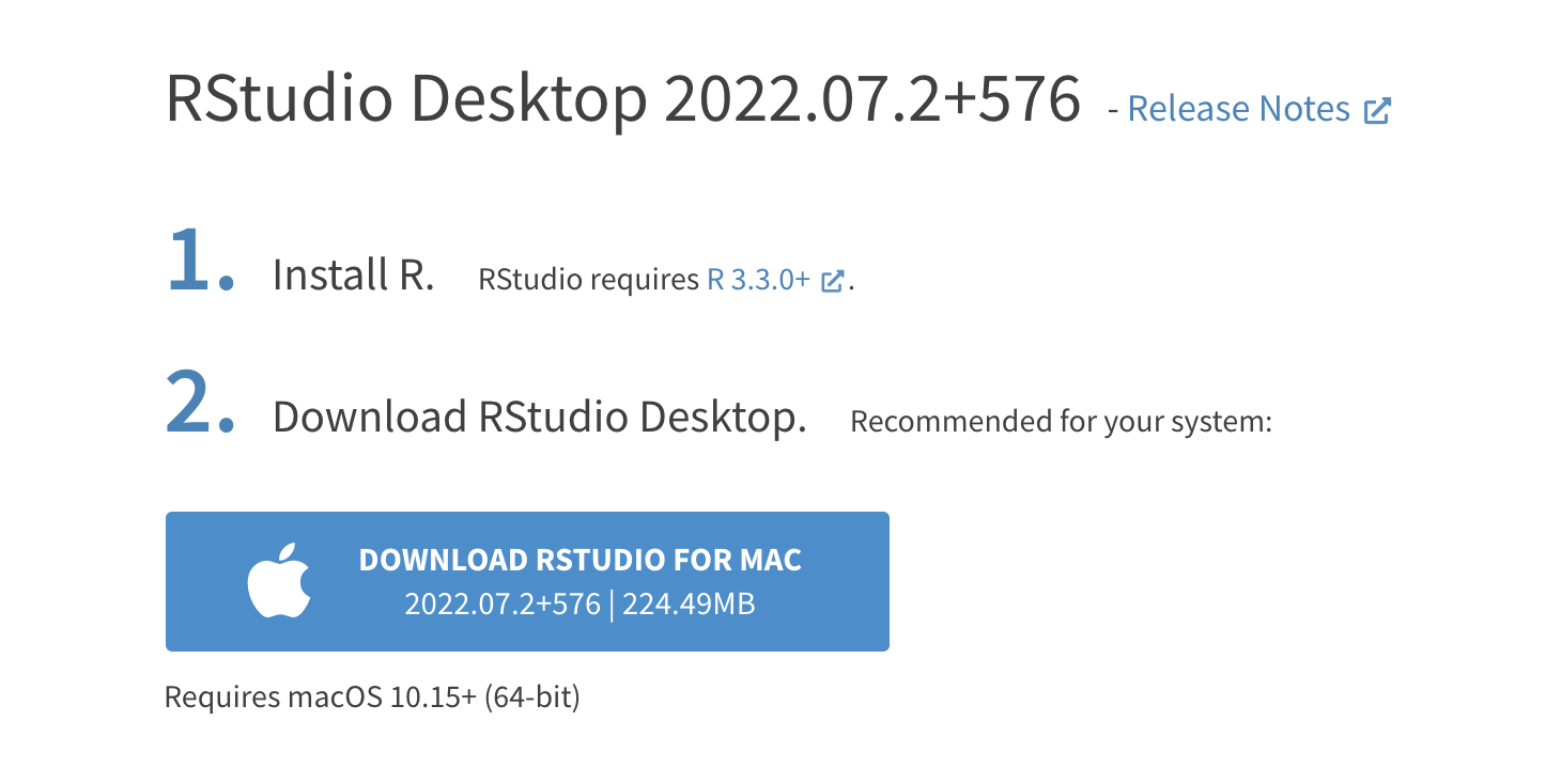
R is free and open source. The Desktop version of RStudio is free.
To use RStudio, you must:

Please feel free to Download the taxa_table.csv and
kraken_all_metasub.csv for your own use.
5. Data Science Principles Covered
- Using commands (e.g.
head,tail) to understand the structure/format of the data. - Use operators (e.g.
$or@) to filter or sort data by specific variables (i.e. columns) - Use commands like ,
summary(),density()andplotto understand the descriptive statistics and general distribution of a dataset. - Dataset sizes (footprints) tend to get smaller as one works through analyses downstream.
- To compare samples visually, one often tries to reduce the dimensionality of the data.
- If you’re having trouble running a command, try to first reproduce the sample code result.
6. Post-VTP Survey
We would greatly appreciate it if you could complete the POST-VTP Survey: https://forms.gle/ogTzjPW61S4WfVou6