
Welcome! If you signed up for the Variant calling with NVIDIA Parabricks and GATK workshop, you're in the right place.
We're taking the first 10 minutes to ensure that you're logged into the MILRD and Deep Origin platforms.
Please:
Login to your Deep Origin account (Username: [ciuser_1], Password: [cipass_1]) and ensure that's it's open in a tab adjacent to this platform so you can easily toggle back and forth. For future reference, you can always find your Deep Origin login info in the Getting Started Channel in the left navigation pane.
Navigate to the Collaborate Channel on the left navigation pane, click on the thread titled "Please Introduce Yourself" and post your name, role, the reason you signed up for this workshop and one non-science fact about you. For example:
Hi, my name is Alice Smith and I'm a scientist a Postdoc at UCSF. I enrolled becuase I'm interested to learn more about variant calling and apply it to my lymphoma research. One non-science fact is that I like to bake becuase it's like a science experiment that almost always works.
If anyone is having issues, please post a question to the Collaborate Channel or Zoom Chat and a mentor from MILRD or Deep Origin will help you.
Variant Calling on Deep Origin + GATK & NVIDIA Parabricks
The goal of this Virtual Training Project (VTP) is to perform variant calling using base GATK & Parabricks GATK, and related tools, on diverse datasets, downstream visualization & analysis, and to discuss analysis considerations.
Using Bash Commands in VSCode, R in RStudio, and Python in Jupyter Notebook, you will be guided step-by-step in:
Single-nucleotide & small-indel variant calling with base GATK and Parabricks GATK on three diverse data types:
PGx Amplicon with ONT (Data source: CariGenetics, Oxford Nanopore Technologies (ONT))
Microbial Whole Genome (Data source: Mason & Venkateswaran Labs, Illumina MiSeq)
Human Tumor vs. Normal Samples Whole Exome (Data Source: SEQC2, Illumina HiSeq 2500)
Downstream visualization & analysis with GATK outputs (e.g. scatterplots, thresholding based on allelic frequency of control sample, etc.)
Variant calling pipeline parameter considerations per data type and experimental constraints
Throughout this VTP, you will have access to:
All required high-performance cloud-compute resources, analysis tools, and software via Deep Origin ComputeBenches
Support from mentors during VTP and 24h afterwards
Access to all source data in the project
Our Approach
This guide is intended as a tool for exploration and learning rather than a strict recipe to follow.
We encourage the sharing of relevant papers and the asking of related questions, particularly in the Collaborate Channel.
We aim to enable participants to start working with data as quickly as possible; this is not intended to be a formal course.
The program is structured to help participants understand the rationale behind each step in the analysis, rather than focusing on the implementation of scalable workflows (e.g. Snakemake) at the outset.
Schedule:
10:00-10:45am PT (1:00-1:45pm ET): Getting Started
10:45-10:55am PT (1:45-1:55pm ET): Break
10:55-11:40am PT (1:55-2:40pm ET): Module 1 - Microbial Whole Genome Variant Calling (Illumina)
11:40am-12:25pm PT (2:40-3:25pm ET): Module 2 - PGx Amplicon Variant Calling (ONT)
12:25-12:35pm PT (3:25-3:35pm ET): Break
12:35-1:20pm PT (3:35-4:20pm ET): Module 3 - Exome Variant Calling in Cancer vs. Normal Sample (Illumina)
1:20-1:30pm PT (4:20-4:30pm ET): Wrap-up and Closing Remarks
Access & Support After the VTP
We are happy to answer questions via this platform's Collaborate Channel for 24 hours after the training is over.
Instructions will be accessible through Friday, March 1, at 5pm PT.
MILRD Platform:
Getting Started Channel: Provides login details for Deep Origin ComputeBench, along with the Assigned Samples/Data IDs for analysis
Instructions Channel: Offers project background, analysis task instructions, AI-enabled question answering, and directs to Collaborate for further assistance when AI responses are inadequate or delayed
Collaborate Channel: Facilitates threaded conversations with mentors and peers on analysis issues and concepts
Results Channel: Enables comparison and discussion of submitted results at instructional Checkpoints (CPs) with those from other participants
If you encounter any issues, follow these steps:
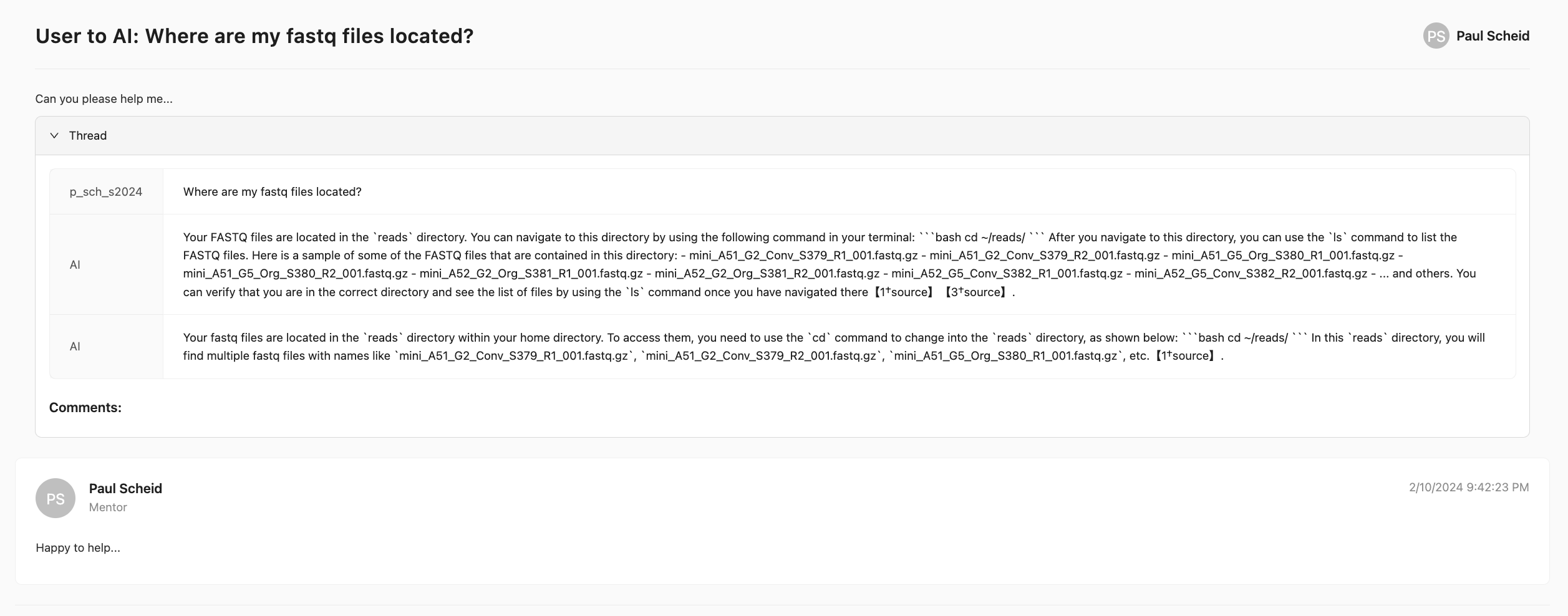
(1) Type your question or paste the error message into the AI question bar and press Enter:
For instance, a participant inquiring about the location of fastq files would enter Where are my fastq files located?:

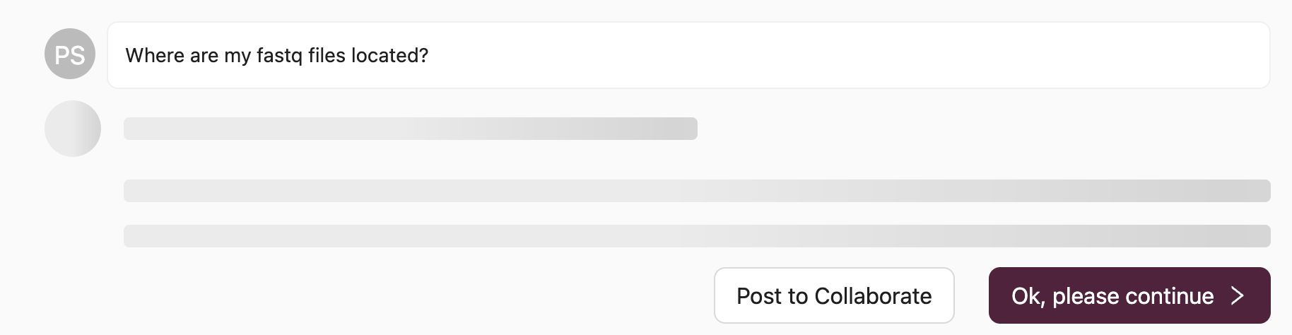
Please note that processing your query may take up to 1 minute. During this time, the platform searches the project's documentation for relevant information, extracts pertinent sections, and utilizes AI for analysis and summarization to provide you with an answer.
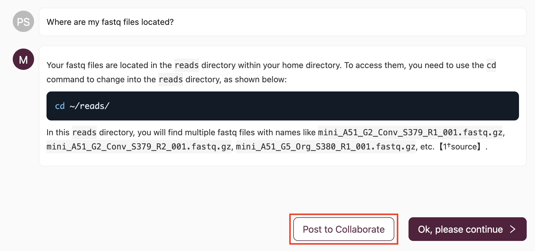
(2) If the response from the AI is helpful but you require further clarification, or if the response is delayed, you have the option to ask another question directly to the AI or use the Post to Collaborate button to seek assistance from a Mentor in the Collaborate Channel:
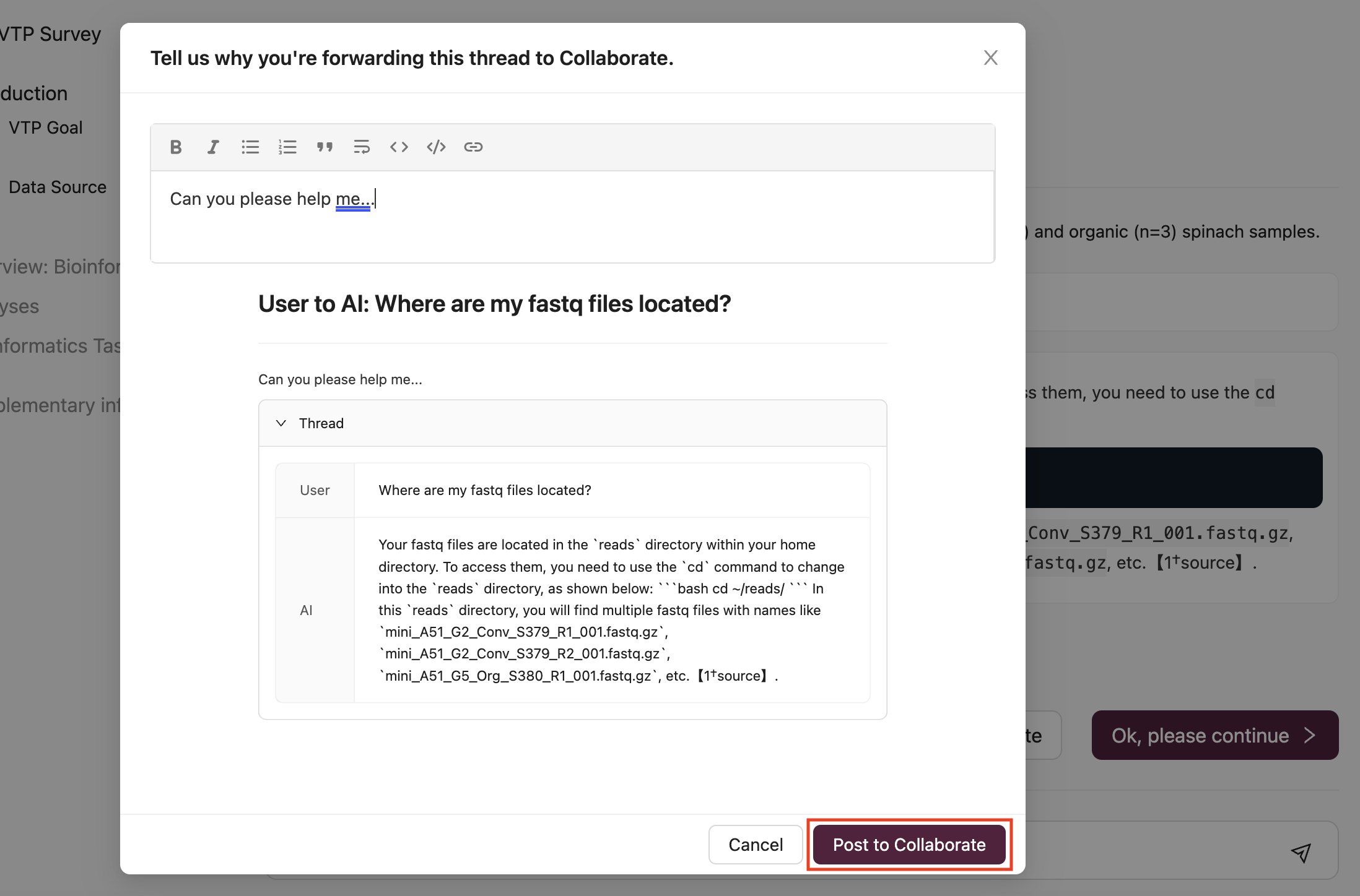
By selecting Post to Collaborate, your question and the AI-generated thread will be shared in the Collaborate Channel:
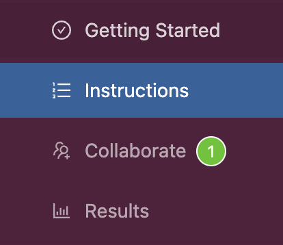
(3) A mentor will then engage with your query in a threaded discussion to provide guidance:
Deep Origin ComputeBench:
Integrated VSCode, RStudio, and Jupyter Notebook within the same AWS-hosted container for seamless analysis
Ability to configure and reconfigure the ComputeBench as needed
Option to set automatic stop times on a ComputeBench to manage resources efficiently
MILRD Mentors:
Preetida (Preeti) Bhetariya, PhD. Preeti is a senior scientist with AstraZeneca in Oncology Data Science. Before switching to pharma, she worked in academia for almost a decade as a Bioinformatics scientist at Dana Farber Cancer Institute and Harvard School of Public Health, where she studied lung cancer using multi-model genomic approaches. Preeti earned her Ph.D. in Biotechnology from the Institute of Genomics and Integrative Biology, India, 2012 in fungal genomics. She did her postdoctoral training at Huntsman Cancer Institute, University of Utah where she developed a bioinformatics pipeline to detect low-frequency variants from circulating tumor DNA during that period. Preeti has more than twelve years of experience in Computational biology, analyzing different NGS modalities, including WGS, WES, RNA-seq, Chip-Seq, scRNA, and scATACseq in the research areas such as autoimmune diseases, infection and immunology, and cancer. She has expertise in single-cell transcriptomics and liquid biopsy genomics. She enjoys building custom analysis workflow with Python and R.
Dmitry Kazantsev, PhD. Dmitry is a postdoctoral researcher at the Institute of Pathological Physiology in Prague, in prof. Klener's lab. His work focuses on multi-omics data acquisition and analysis as a tool for translational hematological oncology.
Miten Jain, PhD. Miten is an Assistant Professor in the Bioengineering department at Northeastern University, with a joint appointment in Physics. His research centers on nanopore technology, single-cell techniques, and computational biology. He received his PhD in Bioinformatics and Biomolecular Engineering from the University of California, Santa Cruz.
Assistant Mentors:
Data Contributors:
All bioinformatics tasks will be conducted in the cloud on your personal Deep Origin ComputeBenches, which are customizable, persistent, and scalable docker-based compute containers running on Amazon Web Services (AWS). These containers come pre-installed with open-source bioinformatics tools and IDEs.
What is cloud computing:
Ensure you are logged in to your Deep Origin account ([ci_1], Username: [ciuser_1], Password: [cipass_1]).
This Virtual Training Project utilizes VSCode, Jupyter Notebook, and RStudio.
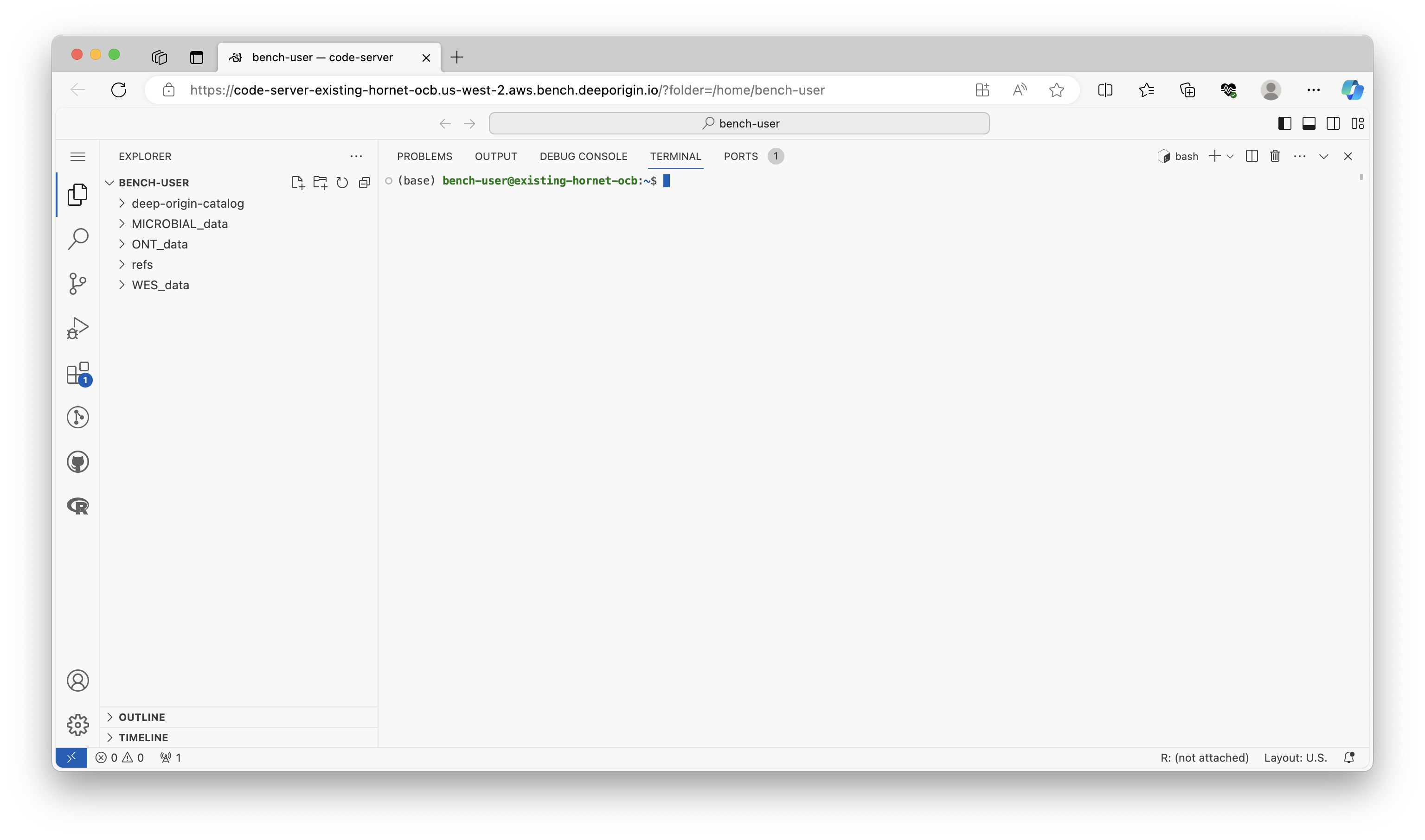
VSCode is a highly extensible code editor that can be configured with plugins to provide many of the features you would expect in an integrated development environment (IDE), such as IntelliSense for smart completions. Here we'll use it to run Linux/Bash commands, but it can be used to support many other programming languages and IDEs. Here's what VSCode looks like after it's configured with the Linux Terminal:
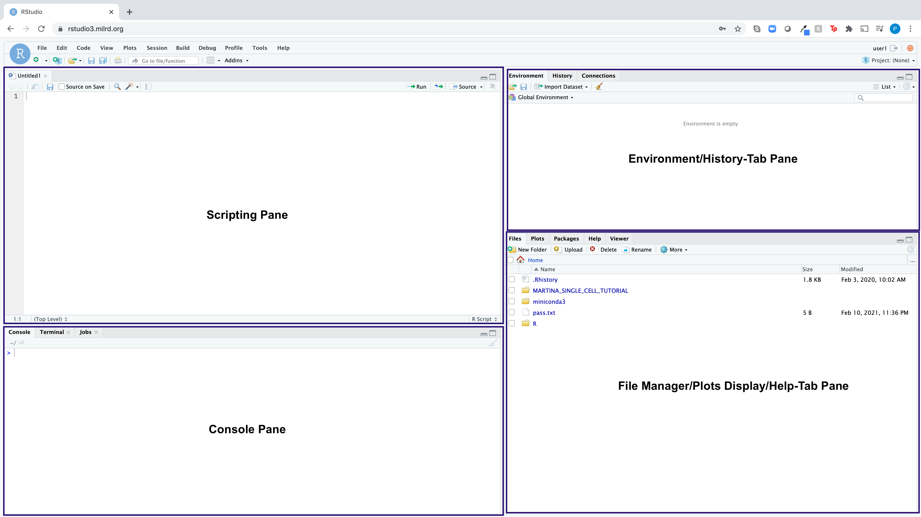
RStudio is an integrated development environment (IDE) for the open-source R programming language, which brings the core components of R (Scripting Pane, Console, Environment Pane, File Manager/Plots/Help Pane) into a quadrant-based user interface for efficient use. Here is what the RStudio dashboard looks like:
Jupyter Notebook is an open-source web application for the Python programming language, providing an interface that integrates the key components of Python (Code Cells, Markdown Cells, Output Area, and Kernel) into a document-like user interface. It allows you to create and share documents that contain live code, equations, visualizations, and narrative text. For more information, you can visit Project Jupyter’s page. Here is what the Jupyter notebook dashboard looks like:

You can always find your Deep Origin login info in the Getting Started Channel.
Navigating your Linux terminal
The first part of each module in this project are performed using the Linux command line in VSCode. Linux is a powerful operating system used by many scientists and engineers to analyze data. Linux commands are written on the command line, which means that you tell the computer what you want it to do by typing, not by pointing and clicking like you do in operating systems like Windows, Chrome, iOS, or macOS. The commands themselves are written in a language called Bash.
Here's a brief tutorial that covers: the accessing the Linux command line in VSCode, Linux command line execution, common commands, and command line structure.
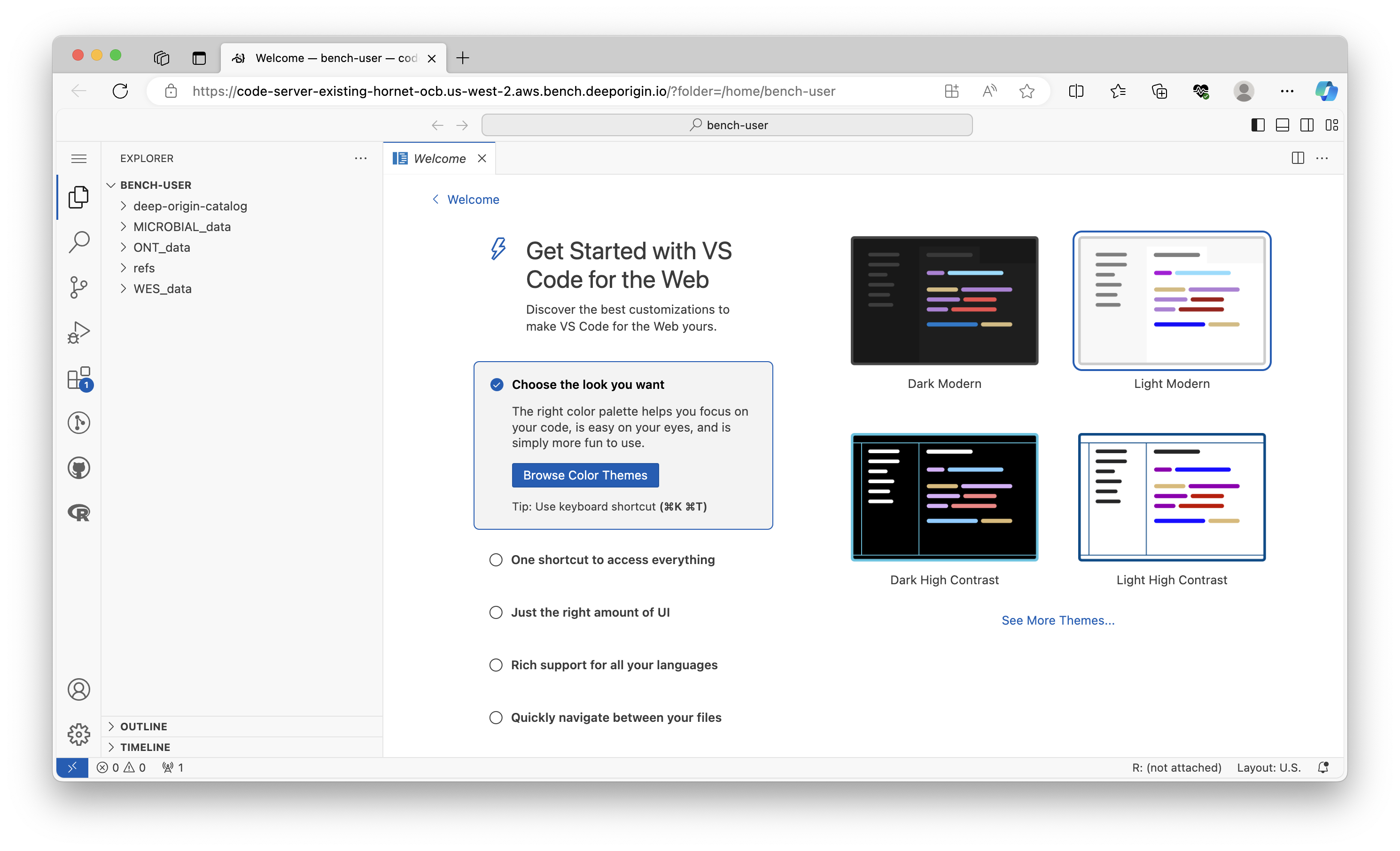
Navigate to your Deep Origin ComputeBench ([ci_1], Username: [ciuser_1], Password: [cipass_1]) and launch VSCode using the Connect button. VSCode will launch in a new tab in your browser:
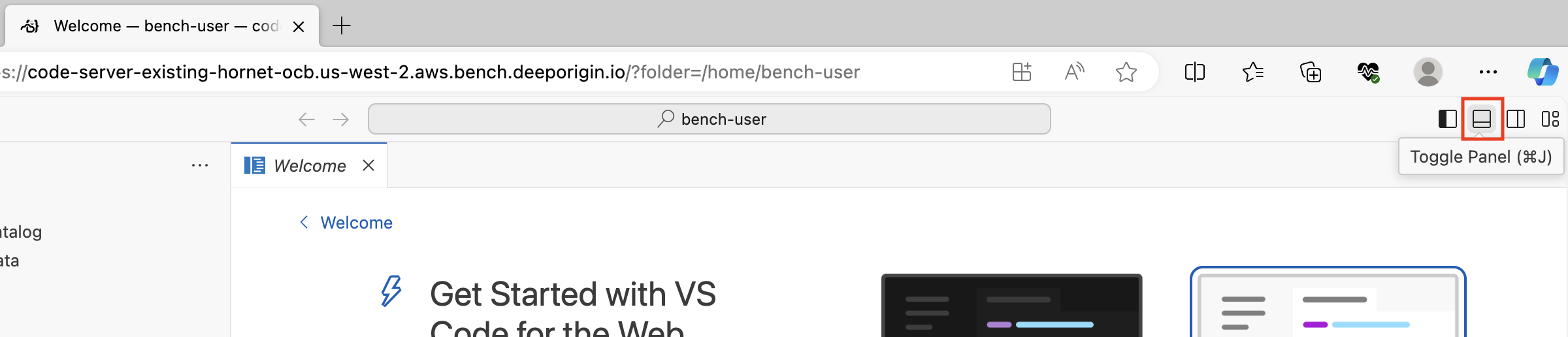
Click the Toggle Panel button in the upper right hand corner:
(Optional) Click the "Maximize Panel Size" button to expand the terminal to fit the full height of the screen:
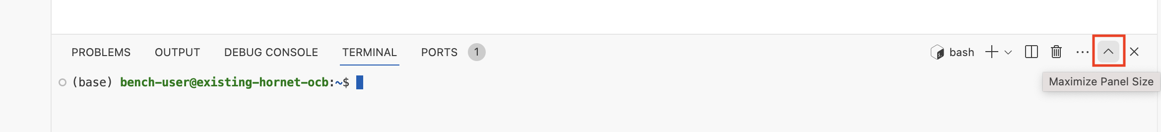
The Linux command line, also known as the terminal, is a text-based interface that allows you to interact with your computer's operating system. The language used to communicate with the terminal is called Bash.
When you open the terminal, you should see something like this:
(base) bench-user@existing-hornet-ocb:~$
(base) bench-user@existing-hornet-ocb:~$ your-command-goes-here
Unlike a graphical user interface (GUI), where you interact with your computer by clicking on icons and buttons, the terminal requires you to type in text commands. While it may take some time to learn the commands and syntax, the terminal can often be faster and more efficient than a GUI for certain tasks.
Let's try a command. The ls command lists the files and directories in the current directory:
ls
The output should look something like this:
deep-origin-catalog MICROBIAL_data ONT_data refs WES_data
The ~ symbol represents the current user's home directory. If you look immediately to the left of the $, you will see the "working directory", which is the directory you are currently in.
To navigate to a different directory, use the cd command. Now, navigate to the MICROBIAL_data directory by typing this command:
cd MICROBIAL_data/
After executing the command, your terminal should look like this:
(base) bench-user@existing-hornet-ocb:~/MICROBIAL_data$
Now, return to the home directory using the cd ~ command:
cd ~
To make a new directory, use the mkdir command. Now make a new directory called test_directory in the current directory:
mkdir test_directory
To confirm that the test_directory directory was created, execute the ls command.
Now navigate into the test_directory directory using the cd command:
cd test_directory
Your terminal should now look like this:
(base) bench-user@existing-hornet-ocb:~/test_directory$
This is a basic introduction to the Linux command line. As you continue with the bioinformatics analyses in this project, you will learn more commands and become more comfortable with the terminal.
Here's a concise list of common Linux commands and their functions:
# File and Directory Management
ls          # Lists files and directories in the current directory
cd <dir>    # Changes the current directory to <dir>
pwd         # Prints the current working directory
mkdir <dir> # Creates a new directory named <dir>
rmdir <dir> # Removes an empty directory named <dir>
rm <file>   # Deletes a file
cp <src> <dest> # Copies a file or directory from <src> to <dest>
mv <src> <dest> # Moves or renames a file or directory

# File Viewing and Editing
cat <file>  # Displays the contents of <file>
less <file> # Views the contents of <file> in a paginated manner
nano <file> # Opens the file <file> in the Nano text editor
vi <file>   # Opens the file <file> in the Vi text editor

# System Information and Management
df          # Displays disk space usage
du          # Shows the disk usage of files and directories
top         # Displays real-time system summary and process info
ps          # Shows information about active processes
kill <pid>  # Terminates the process with process ID <pid>

# Networking
ping <host> # Sends ICMP ECHO_REQUEST to network hosts
ifconfig    # Configures and displays network interface parameters
ssh <host>  # Connects to <host> via SSH
scp <src> <dest> # Copies files between hosts on a network

# Searching and Sorting
grep <pattern> <file> # Searches for <pattern> in <file>
find <dir> -name <name> # Finds files or directories within <dir> with name <name>
sort <file> # Sorts lines in <file>
uniq <file> # Filters out repeated lines in <file>

# Compression and Archiving
tar -cvf <archive.tar> <dir> # Creates an archive file from <dir>
tar -xvf <archive.tar>       # Extracts files from an archive
gzip <file>  # Compresses <file> using gzip
gunzip <file.gz> # Decompresses <file.gz>

# File Permissions
chmod <mode> <file> # Changes the permission of <file> to <mode>
chown <user>:<group> <file> # Changes the owner and group of <file>
Linux commands typically follow a consistent structure, regardless of their length. The general structure is:
command [options] [arguments]
ls, grep, or cp.-) or double hyphen (--).Examples
Short Command
ls
Medium Length Command
grep -i "example" file.txt
grep (searches for patterns within files)
Option: -i (ignore case during search)
Argument: "example" (the pattern to search for), file.txt (the file to search in)
Long Command
tar -czvf archive.tar.gz /path/to/directory
tar (creates or extracts archives)
Options: -czvf
Arguments: archive.tar.gz (name of the archive file to create), /`path/to/directory`` (the directory to archive)
In all these examples, the basic structure of the command remains consistent: the command itself, followed by any options (if needed), and then the arguments (if any). This uniform structure makes it easier to understand and predict how to construct and use various Linux commands.
Intro to Python
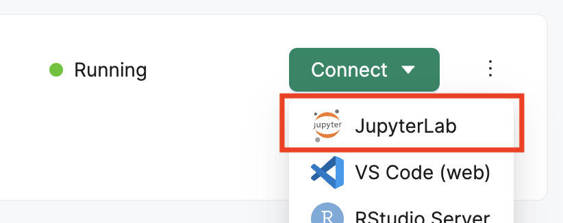
Navigate to your Deep Origin ComputeBench ([ci_1], Username: [ciuser_1], Password: [cipass_1]) and launch JupyterLab using the Connect button. JupyterLab will open in a new tab in your browser:
Once JupyterLab is open, you can create a new Jupyter Notebook by clicking on the first option in the Launcher (Outlined in red):
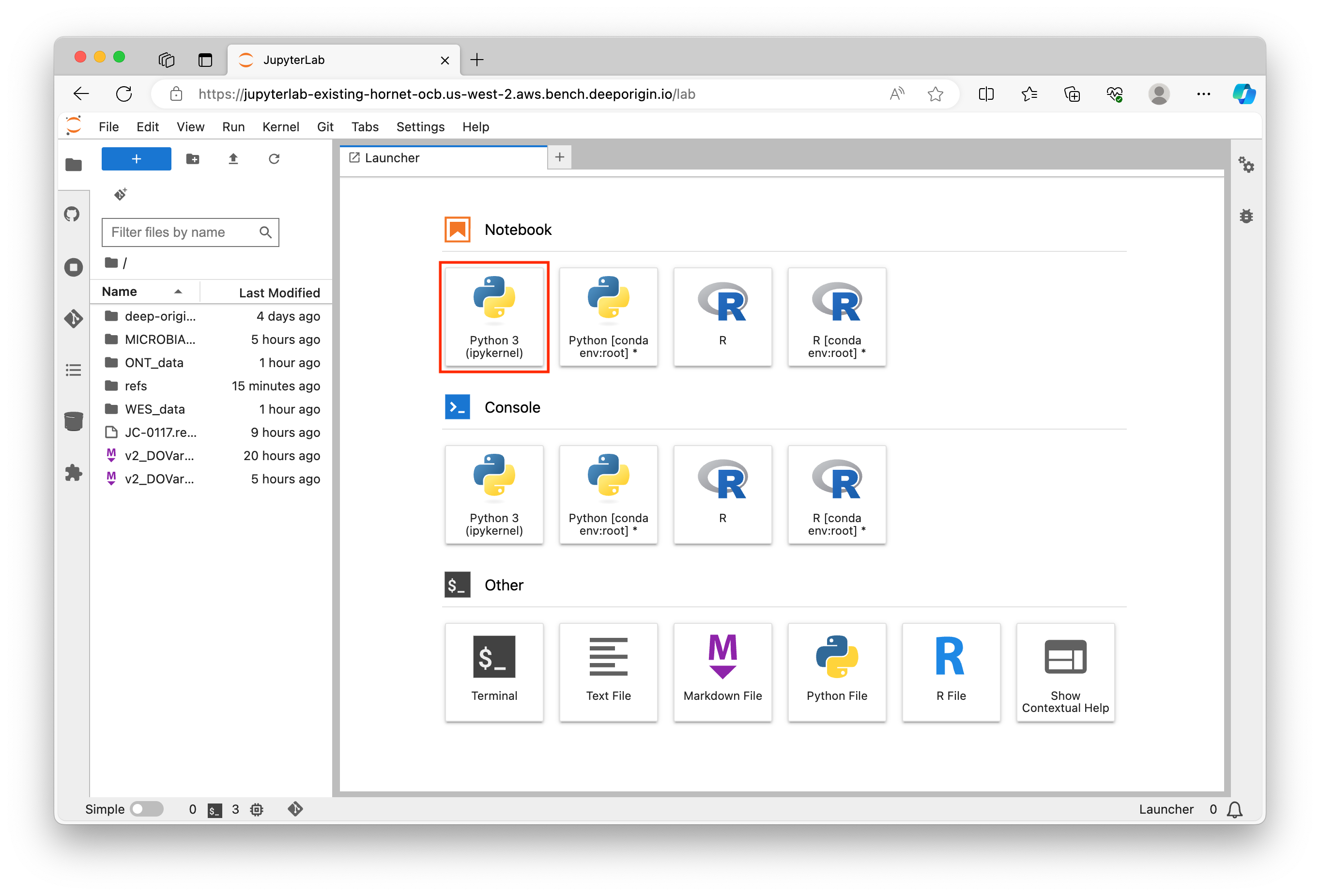
A new notebook will open where you can start writing your Python code. You can enter Python commands in the cells provided and execute them by pressing Shift + Enter (or the play button):
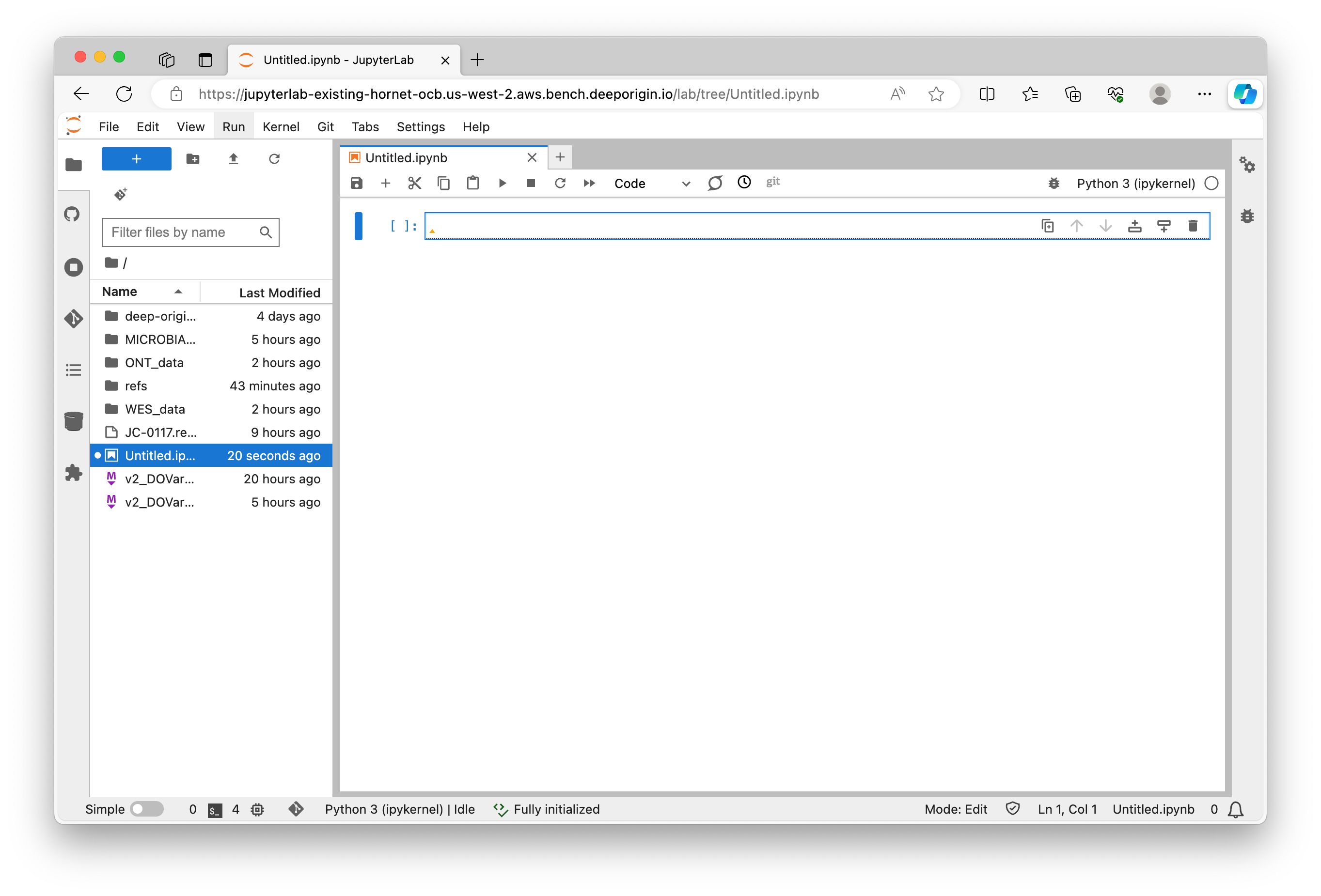
Jupyter Notebook is an interactive computing environment that enables users to create notebook documents that include live code, narrative text, equations, and visualizations.
When you create a new notebook, you'll see a cell where you can start typing Python code immediately. Here's an example of a simple Python command:
print("Hello, World!")
Shift + Enter to execute the cell and you should see the output below the cell:
Hello, World!
Jupyter Notebooks are great for data analysis and visualization. You can import libraries such as numpy, pandas, matplotlib, and seaborn to help with these tasks. Here's an example of importing a library and using it to create a simple plot:
import matplotlib.pyplot as plt
plt.plot([1, 2, 3, 4])
plt.ylabel('some numbers')
plt.show()
You can also use Markdown cells to add narrative text to your notebook. To create a Markdown cell, click on the dropdown menu in the toolbar and select Markdown. Then, you can type your text and format it using Markdown syntax. To execute the Markdown cell, press Shift + Enter.
Jupyter Notebooks are powerful tools for combining code, output, and narrative into a single document. They are widely used in data science to create reproducible analyses and share results with others.
Here's a concise list of common Python commands and their functions:
# Basic Python Commands
print("Hello, World!")  # Prints a string to the console
for i in range(5):      # Loops over a range of numbers
    print(i)

# Importing Libraries
import numpy as np      # Imports the numpy library as np
import pandas as pd     # Imports the pandas library as pd

# Data Analysis and Visualization
df = pd.read_csv('data.csv')  # Reads a CSV file into a pandas DataFrame
df.head()                      # Displays the first five rows of the DataFrame
df.describe()                  # Generates descriptive statistics of the DataFrame

plt.figure(figsize=(10,6))     # Sets the figure size for a plot
plt.hist(df['column_name'])    # Creates a histogram of a specified column
plt.show()                     # Displays the plot
These are just a few examples of the many commands you can use in Python. As you work with Jupyter Notebooks, you'll learn more about Python's extensive libraries and capabilities for data analysis and visualization.
Intro to R
RStudio is an integrated development environment (IDE) for R, a programming language for statistical computing and graphics. RStudio makes it easier to write R code and includes tools for plotting, history, debugging, and workspace management.
Here's a brief tutorial that covers: accessing RStudio, RStudio interface, common commands, and R script execution.
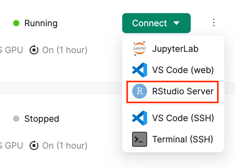
Navigate to your Deep Origin ComputeBench ([ci_1], Username: [ciuser_1], Password: [cipass_1]) and launch RStudio using the Connect button. RStudio will launch in a new tab in your browser:
Once RStudio is open, you will see the RStudio interface, which is divided into several panes:

The Console pane is where R code is executed. You can type commands directly into the console and press Enter to run them.
The Script pane is where you can write and edit R scripts. Scripts are simply text files with the .R extension that contain a series of R commands.
To run a command from the Script pane, place your cursor on the line of code and press Ctrl + Enter. The command will be executed in the Console pane, and the output will be displayed there.
The RStudio interface is designed to make it easy to write, edit, and run R code. It consists of several key components:
When you start RStudio, the console will display a prompt (>) indicating that it is ready to accept commands. You can type R commands directly into the console and press Enter to execute them.
To create a new R script, go to File > New File > R Script. This will open a new tab in the Script Editor pane where you can write your code.
To save your script, go to File > Save or File > Save As... and choose a location on your computer.
To run your entire script, press the Source button on the top right of the Script Editor pane. This will execute all the commands in the script and display the output in the Console pane.
Here's a concise list of common R commands and their functions:
# Basic R Commands
print("Hello, World!")  # Prints a string to the console
for(i in 1:5) {         # Loops over a range of numbers
  print(i)
}

# Importing Libraries
library(ggplot2)        # Loads the ggplot2 library

# Data Analysis and Visualization
data(mpg)               # Loads the mpg dataset
head(mpg)               # Displays the first six rows of the dataset
summary(mpg)            # Generates descriptive statistics of the dataset

ggplot(mpg, aes(displ, hwy, colour = class)) +
  geom_point()          # Creates a scatter plot
These are just a few examples of the many commands you can use in R. As you work with RStudio, you'll learn more about R's extensive libraries and capabilities for data analysis and visualization.
Executing R scripts in RStudio is straightforward. Here's the general process:
Ctrl + Enter.Source button at the top of the Script Editor pane.R scripts can also include comments, which are lines that are not executed and are used to explain the code. Comments in R start with the # symbol.
Variant calling is a bioinformatics process used to identify variations such as single nucleotide polymorphisms (SNPs), insertions, deletions, and structural variants in a genome. This process is crucial in many fields such as genomics, population genetics, and medical genetics. Here are some key concepts related to variant calling:
Mismatch: A mismatch is a difference between the sequences of the same gene in different individuals. It can be a single nucleotide difference (SNP) or a longer sequence difference.
Paired-end vs. Single-end reads: In paired-end sequencing, both ends of the DNA fragment are sequenced, whereas in single-end sequencing, only one end is sequenced. Paired-end sequencing allows for more accurate alignment and detection of structural variants. It also helps in identifying PCR duplicates. If multiple reads have the same start and end points, they are likely duplicates from PCR amplification.
Read Depth: Read depth refers to the number of times a particular base is read during sequencing. A higher read depth increases the confidence in the call made at that position a variant calling algorithm.
PCR Duplicates: During the preparation of sequencing libraries, the same DNA molecule can be sequenced multiple times, leading to duplicates. These duplicates can bias the variant calling process and are usually removed before variant calling.
Phasing: Phasing is the process of determining which variants occur on the same DNA molecule. It is important for understanding the biological effects of variants.
Read Length: Read length is the number of base pairs sequenced from a single read. Longer read lengths can improve the accuracy of alignment and variant calling, but they may also increase the error rate.
Here are some tools commonly used in variant calling:
GATK: The Genome Analysis Toolkit (GATK) is a software package developed by the Broad Institute to analyze high-throughput sequencing data. GATK is widely used for variant discovery in germline and somatic data.
NVIDIA Parabricks GATK: NVIDIA Parabricks is a computational framework that uses graphics processing units (GPUs) to accelerate the analysis of sequence data. It includes a version of GATK optimized for GPUs.
Clair3: Clair3 is a variant calling tool designed for long-read sequencing data. It can call single nucleotide variants, insertions and deletions, and large structural variants.
Samtools: Samtools is a suite of programs for interacting with high-throughput sequencing data. It includes utilities for variant calling and alignment.
Picard: Picard is a set of Java-based command-line utilities for manipulating high-throughput sequencing data.
Minimap2: Minimap2 is a versatile sequence alignment program that aligns DNA or mRNA sequences against a large reference database.
DeepVariant: DeepVariant is a tool developed by Google that uses deep learning to call genetic variants from next-generation DNA sequencing data.
For more detailed information on best practices for variant calling, refer to the GATK Best Practices guide here.
Background
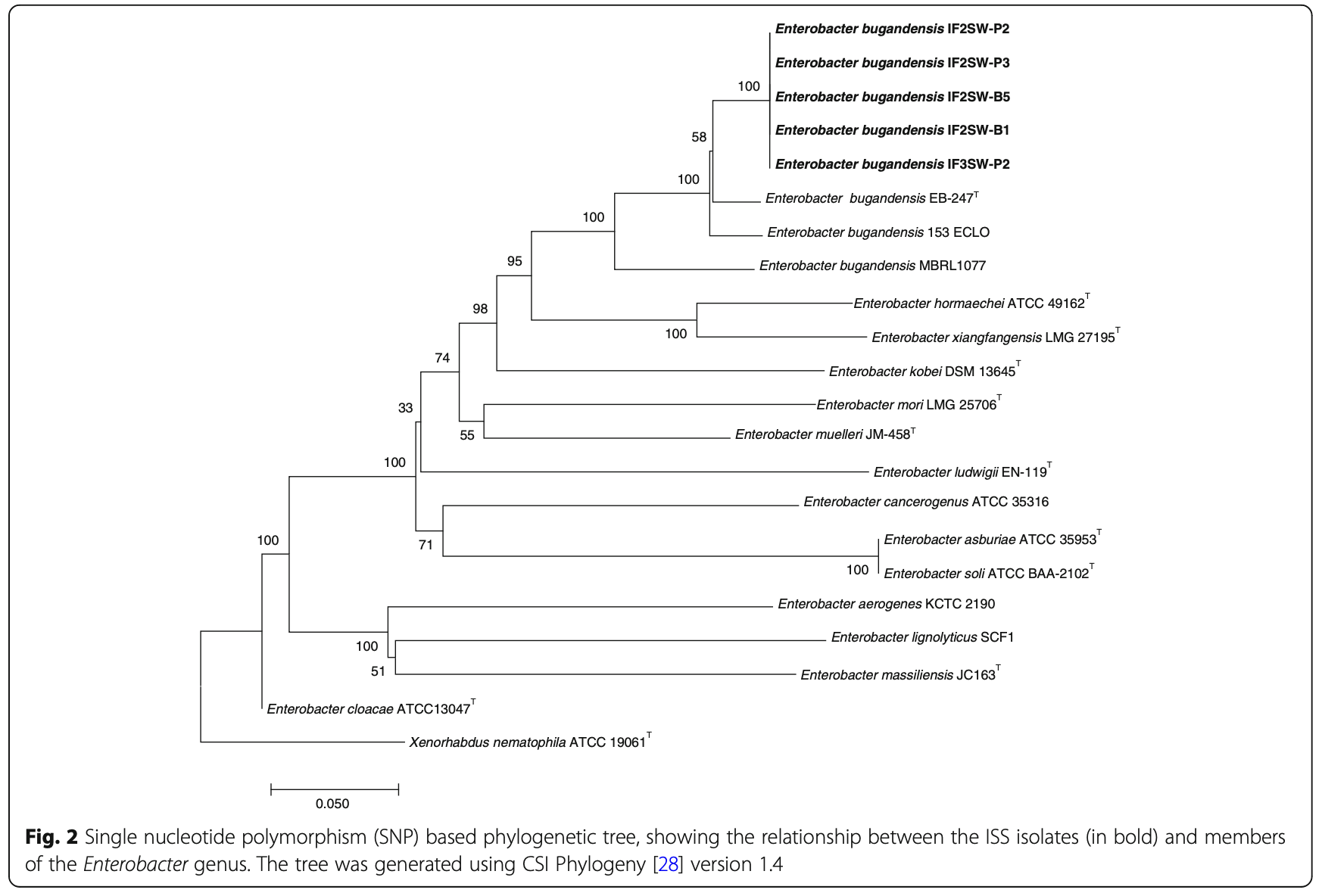
The focus of this analysis is derived from the study of five Enterobacter bugandensis strains isolated from the International Space Station (ISS). These strains were examined for antimicrobial resistance (AMR) phenotypes, multiple drug resistance (MDR) gene profiles, and genes related to potential virulence and pathogenic properties, and compared with three clinical strains. The study utilized a hybrid de novo assembly of Nanopore and Illumina reads for whole genome sequencing. The full abstract of the research paper can be accessed here.
Analysis Goals
The goal of this analysis is to perform variant calling on the whole genome sequencing data of the ISS strains to identify genetic variants and perform phylogenetic analysis to compare the ISS strains to their eartbound counterparts.
Considerations
Analysis Plan
The analysis will involve the following steps:
Sample Information
The samples used in this analysis are derived from different microbial strains collected from the ISS. The identifiers and corresponding strain names are as follows:
For more details on the analysis, refer to Figure 2 of the research paper:
Analyze Example Sample JC-0117 (IF2SW-P3):
conda install picard
Build the reference genome
samtools faidx ~/refs/GCF_002890725.1_ASM289072v1_genomic.fa
gatk CreateSequenceDictionary \
    -R ~/refs/GCF_002890725.1_ASM289072v1_genomic.fa \
    -O ~/refs/GCF_002890725.1_ASM289072v1_genomic.dict
(Unmapped .bam file is created from .fastq reads. This file will be required at a later stage.)
You will need read group information which can be found in the .fastq file header:
.fastq File Formats
Latest release .fastq file identifier format:
@Instrument:RunID:FlowCellID:Lane:Tile:X:Y ReadNum:FilterFlag:0:SampleNumber
@A00814:76:HNLLGDSXX:1:1101:28302:1000
Mapping the new version fields to our fastq identifier:
@Instrument: @A00814
RunID:76
FlowCellID: HNLLGDSXX
Lane:1
Tile:1101
X:28302
Y 1000
More information on .fastq file format can be found here.
FastqToSam
SKIP THIS STEP FOR THIS VTP: we have provided the output of this step in the interest of time.
gatk FastqToSam \
    FASTQ=~/MICROBIAL_data/fastq/JC-0117_S1047_L001_R1_001.fastq.gz \
    FASTQ2=~/MICROBIAL_data/fastq/JC-0117_S1047_L001_R2_001.fastq.gz \
    OUTPUT=~/MICROBIAL_data/JC-0117.unmapped.bam \
    READ_GROUP_NAME=HNLLGDSXX:1 \
    SAMPLE_NAME=JC-0117 \
    LIBRARY_NAME=Solexa-272222 \
    PLATFORM_UNIT=HNLLGDSXX \
    PLATFORM=illumina
.fasta fileMicrobial species can have variable ploidy and closed circular genomes. When circular genomes are sequenced, artificial breakpoints are introduced to linearize the genome for read matching purposes. Hence, any reads spanning the artifical breakpoints are lost. For solving this, ShiftFasta shifts the reference genome 180 degree to move the artificial breakpoint to other location, and call the variants.
ShiftFasta
gatk --java-options "-Xmx2500m" ShiftFasta \
    -R ~/refs/GCF_002890725.1_ASM289072v1_genomic.fa \
    -O ~/refs/GCF_002890725.1_ASM289072v1_genomic.fa.shifted.fasta \
    --interval-file-name ~/refs/GCF_002890725.1_ASM289072v1_genomic.fa \
    --shift-back-output ~/refs/GCF_002890725.1_ASM289072v1_genomic.fa.shiftback.chain
This creates an index of the shifted reference genome for efficient alignment.
bwa index
bwa index ~/refs/GCF_002890725.1_ASM289072v1_genomic.fa.shifted.fasta
bwa mem
bwa mem -K 100000000 -v 3 -t 16 -Y \
    ~/refs/GCF_002890725.1_ASM289072v1_genomic.fa.shifted.fasta \
    ~/MICROBIAL_data/fastq/JC-0117_S1047_L001_R1_001.fastq.gz \
    ~/MICROBIAL_data/fastq/JC-0117_S1047_L001_R2_001.fastq.gz \
    > >(tee JC-0117.realigned.bwa.stderr.log >&2) \
    > ~/MICROBIAL_data/JC-0117.unmapped.realigned.bam
Aligns sequencing reads to the shifted reference genome.
MergeBamAlignment
SKIP THIS STEP FOR THIS VTP: we have provided the output of this step in the interest of time.
picard MergeBamAlignment \
    VALIDATION_STRINGENCY=SILENT \
    EXPECTED_ORIENTATIONS=FR \
    ATTRIBUTES_TO_RETAIN=X0 \
    ATTRIBUTES_TO_REMOVE=NM \
    ATTRIBUTES_TO_REMOVE=MD \
    ALIGNED_BAM=~/MICROBIAL_data/JC-0117.unmapped.realigned.bam \
    UNMAPPED_BAM=~/MICROBIAL_data/JC-0117.unmapped.bam \
    OUTPUT=~/MICROBIAL_data/mba.bam \
    REFERENCE_SEQUENCE=~/refs/GCF_002890725.1_ASM289072v1_genomic.fa \
    PAIRED_RUN=true \
    SORT_ORDER="unsorted" \
    IS_BISULFITE_SEQUENCE=false \
    ALIGNED_READS_ONLY=false \
    CLIP_ADAPTERS=false \
    MAX_RECORDS_IN_RAM=2000000 \
    ADD_MATE_CIGAR=true \
    MAX_INSERTIONS_OR_DELETIONS=-1 \
    PRIMARY_ALIGNMENT_STRATEGY=MostDistant \
    PROGRAM_RECORD_ID="bwamem" \
    PROGRAM_GROUP_VERSION="~{bwa_version}" \
    PROGRAM_GROUP_COMMAND_LINE="~{bwa_commandline}" \
    PROGRAM_GROUP_NAME="bwamem" \
    UNMAPPED_READ_STRATEGY=COPY_TO_TAG \
    ALIGNER_PROPER_PAIR_FLAGS=true \
    UNMAP_CONTAMINANT_READS=true \
    ADD_PG_TAG_TO_READS=false
MarkDuplicates
picard MarkDuplicates \
    INPUT=~/MICROBIAL_data/mba.bam \
    OUTPUT=~/MICROBIAL_data/md.bam \
    METRICS_FILE=metric.txt \
    VALIDATION_STRINGENCY=SILENT \
    OPTICAL_DUPLICATE_PIXEL_DISTANCE=2500 \
    ASSUME_SORT_ORDER="queryname" \
    CLEAR_DT="false" \
    ADD_PG_TAG_TO_READS=false
Marks duplicates in the BAM file.
SortSam
picard SortSam \
    INPUT=~/MICROBIAL_data/md.bam \
    OUTPUT=~/MICROBIAL_data/JC-0117.realigned.sorted.bam \
    SORT_ORDER="coordinate" \
    CREATE_INDEX=true \
    MAX_RECORDS_IN_RAM=300000
Sorts the .bam file by genomic coordinates.
Inputs: .bam file with duplicates marked.
Output: Sorted .bam file.
Performs variant calling using Mutect2.
Mutect2
Mutect2 (GATK somatic) is used for microbial variant calling.
gatk Mutect2 \
    -R ~/refs/GCF_002890725.1_ASM289072v1_genomic.fa.shifted.fasta \
    -I ~/MICROBIAL_data/JC-0117.realigned.sorted.bam \
    -O ~/MICROBIAL_data/JC-0117.realigned_shifted.vcf \
    --annotation StrandBiasBySample \
    --num-matching-bases-in-dangling-end-to-recover 1 \
    --max-reads-per-alignment-start 75
.bam file..vcf file.Lifts over the .vcf file back to the original reference coordinates.
LiftoverVcf
picard LiftoverVcf \
    I=~/MICROBIAL_data/JC-0117.realigned_shifted.vcf \
    O=~/MICROBIAL_data/JC-0117.shifted_back.vcf \
    R=~/refs/GCF_002890725.1_ASM289072v1_genomic.fa.shifted.fasta \
    CHAIN=~/refs/GCF_002890725.1_ASM289072v1_genomic.fa.shiftback.chain \
    REJECT=~/MICROBIAL_data/JC-0117.rejected.vcf
.vcf file, Reference genome, Chain file..vcf file, Rejected variants file.MergeVcfs
picard MergeVcfs \
    I=~/MICROBIAL_data/JC-0117.shifted_back.vcf \
    I=~/MICROBIAL_data/JC-0117.unshifted.vcf \
    O=~/MICROBIAL_data/JC-0117.final.vcf
Merges multiple .vcf files into one.
.vcf file and Shifted .vcf file.vcf file.Download a file necessary for the next step:
AWS_ACCESS_KEY_ID=AKIAZMZLFZJDOPONJ6HB AWS_SECRET_ACCESS_KEY=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 s5cmd sync s3://deeporigin-vtp/vtp-archive/MICROBIAL_data/JC-0117.realigned_shifted.vcf.stats /home/bench-user/MICROBIAL_data/
gatk MergeMutectStats \
    --stats ~/MICROBIAL_data/JC-0117.unshifted.vcf.stats \
    --stats ~/MICROBIAL_data/JC-0117.realigned_shifted.vcf.stats \
    -O ~/MICROBIAL_data/JC-0117.final.combined.stats
.vcf file..vcf file.Filters calls made by Mutect2.
FilterMutectCalls
gatk FilterMutectCalls \
    -V ~/MICROBIAL_data/JC-0117.final.vcf \
    -R ~/refs/GCF_002890725.1_ASM289072v1_genomic.fa \
    -O ~/MICROBIAL_data/JC-0117.final.filtered.vcf \
    --stats ~/MICROBIAL_data/JC-0117.final.combined.stats \
    --microbial-mode
.vcf file..vcf file.Reverts any modifications made during processing and alignment.
Phylogeny
mafft --ep 0.123 --auto ~/refs/Enterobacter_speceis_IF2SW_phylogeny.fa > ~/MICROBIAL_data/Enter_mergerd.output
Visulize phylogenetic tree using NJ / UPGMA phylogeny:
Enter_mergerd.output as input to run NJ algorithm on multiple alignment.Note on Parabricks and Microbial GATK
It is not possible to perform the Microbial GATK pipeline on NVIDIA Parabricks.
Please answer:
1. What special considerations go into variant calling with microbes?
Background:
CariGenetics has performed the Twist Alliance Long Read Pharmacogenetics (PGx) Panel, designed originally for PacBio, on the Oxford Nanopore Technologies (ONT) P48 machine. This ONT Twist PGx panel includes 49 genes, including all the CYP genes (i.e CYP1A2, CYP2B6, CYP2C19, CYP2C8, CYP2C9, CYP2D6, CYP3A4, CYP3A5 and CYP4F2), and all 20 genes with Clinical Pharmacogenetics Implementation Consortium (CPIC) Guidelines. The data comes from 4 people of diverse ethnicities, usually underrepresented in genomic datasets.
PGx is the study of how genes affect a person’s response to therapeutic drugs. Approximately 99% of adults have an actionable PGx variant (from US & UK Biobank studies), approximately 50% of US adults are prescribed a drug for which there are CPIC guidelines, and there are more than 100,000 adverse drug reactions per year in the US costing more than $30 billion dollars.
By performing this one-time PGx test, a person can know which drugs to take the first time, instead of going through a trial-and-error approach which wastes resources, time and negatively impacts care.
A good example of a drug prescription decision that can be impacted by PGx results is codeine. A common drug used for pain relief, codeine is a prodrug that is not active until it reaches the liver and it is converted into morphine. This is metabolised by the CPY2D6 enzyme. According to CPIC guidelines, if the results reveal either of two extreme genotypes——ultrarapid metabolizer or poor metabolizer——the recommendation is to avoid codeine use, either for potential serious toxicity or possibility of diminished pain relief, respectively.
Analysis Goals
minimap2, clair3, and deepvariant for alignment and variant callingConsiderations
CYP1A2 (ENSG00000140505), CYP2B6 (ENSG00000197408), CYP2C19 (ENSG00000165841), CYP2C8 (ENSG00000138115), CYP2C9 (ENSG00000138109), CYP2D6 (ENSG00000100197), CYP3A4 (ENSG00000160868), CYP3A5 (ENSG00000106258), CYP4F2 (ENSG00000185499), HLA-A (ENSG00000206503), HLA-B (ENSG00000234745), HLA-DQA1 (ENSG00000204287), HLA-DRB1 (ENSG00000196126), ABCB1 (ENSG00000085563), ABCG2 (ENSG00000118777), ADD1 (ENSG00000148400), ADRA2A (ENSG00000150594), ANKK1 (ENSG00000198663), APOL1 (ENSG00000174808), BCHE (ENSG00000114200), CACNA1S (ENSG00000036828), CFTR (ENSG00000001626), COMT (ENSG00000093010), CTBP2P2 (ENSG00000235746), DPYD (ENSG00000188641), DRD2 (ENSG00000149295), F2 (ENSG00000180210), F5 (ENSG00000198734), G6PD (ENSG00000160211), GBA (ENSG00000177628), GRIK4 (ENSG00000145864), HTR2C (ENSG00000147246), IFNL3 (ENSG00000164136), MT-RNR1 (ENSG00000211459), MTHFR (ENSG00000177000), NAGS (ENSG00000141552), NAT2 (ENSG00000156006), NUDT15 (ENSG00000162591), OPRD1 (ENSG00000112038), OPRK1 (ENSG00000136854), OPRM1 (ENSG00000112038), POLG (ENSG00000140521), RYR1 (ENSG00000196218), SLC6A4 (ENSG00000108576), SLCO1B1 (ENSG00000134538), TPMT (ENSG00000137364), UGT1A1 (ENSG00000241635), UGT2B15 (ENSG00000171234), VKORC1 (ENSG00000167323), YEATS4 (ENSG00000124356)
Step 1: Alignment with minimap2
minimap2 \
    -ax map-ont \
    -t 4 \
    ~/refs/Homo_sapiens_assembly38.fasta \
    ~/ONT_data/fastq/fastq_runid_7c299c5f19bd1502f6745a5c07d438f287c804ab_1000_0.fastq \
| samtools sort \
    -o ~/ONT_data/runid_7c299c5f19bd1502f6745a5c07d438f287c804ab_1000_aligned.bam
Explanation of Parameters:
-ax map-ont: This option specifies the preset for Oxford Nanopore Technologies (ONT) reads.-t 4: This option specifies the number of threads to use in the alignment process. More threads will make the computation faster but will use more computational resources.~/refs/Homo_sapiens_assembly38.fasta: This is the reference genome file. It is a FASTA file which contains the reference genome sequence.~/ONT_data/fastq/fastq_runid_7c299c5f19bd1502f6745a5c07d438f287c804ab_1000_0.fastq: This is the input file for minimap2. It is a FASTQ file which contains the sequencing reads.| samtools sort: This command is used to sort the output of minimap2.-o ~/ONT_data/runid_7c299c5f19bd1502f6745a5c07d438f287c804ab_1000_aligned.bam: This is the output file for the sorted alignment. It is a BAM file which contains the sorted aligned sequencing reads.Step 2: Create Index for .bam file
samtools index ~/ONT_data/runid_7c299c5f19bd1502f6745a5c07d438f287c804ab_1000_aligned.bam
Step 3: Variant Calling with clair3
In the interest of time, we're going to skip the next step (variant calling with clair3) and provide the pre-processed vcf file instead:
To save time, we'll skip the variant calling step (clair3) and directly provide the pre-processed VCF file output:
AWS_ACCESS_KEY_ID=AKIAZMZLFZJDOPONJ6HB AWS_SECRET_ACCESS_KEY=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 s5cmd sync s3://deeporigin-vtp/vtp-archive/ONT_data/runid_7c299c5f19bd1502f6745a5c07d438f287c804ab_1000 /home/bench-user/ONT_data/
clair3 \
    --bam_fn=/home/bench-user/ONT_data/runid_7c299c5f19bd1502f6745a5c07d438f287c804ab_1000_aligned.bam \
    --ref_fn=/home/bench-user/refs/Homo_sapiens_assembly38.fasta \
    --output=/home/bench-user/ONT_data/runid_7c299c5f19bd1502f6745a5c07d438f287c804ab_1000 \
    --threads=4 \
    --platform=ont \
    --model_path=/home/bench-user/.apps/conda/envs/clair3/bin/models/ont \
    --haploid_precise
clair3 takes ~30 minutes with 4 threads. You're welcome to try it after the VTP.
Explanation of Parameters:
* --bam_fn: This is the input file for clair3. It is a .bam file which contains the aligned sequencing reads.
* --ref_fn: This is the reference genome file. It is a .fasta file which contains the reference genome sequence.
* --output: This is the directory where clair3 will write its output files.
* --threads: This is the number of threads that clair3 will use for its computation. More threads will make the computation faster but will use more computational resources.
* --platform: This specifies the sequencing platform. In this case, it is set to 'ont' which stands for Oxford Nanopore Technologies.
* --model_path: This is the path to the model file that clair3 will use for variant calling.
* --haploid_precise: This is a flag that tells clair3 to perform haploid precise variant calling.
Step 4: Visualize Results in Python IGV
Now we'll visualize these result using Integrative Genomics Viewer (IGV) via the igv-notebook python library in a Jupyter notebook. IGV is a visualization tool developed by the Broad Institute. It allows users to simultaneously integrate and analyze multiple types of genomic data. For more information, you can visit the Broad Institute’s IGV page.
Open the ONT_IGV_viz.ipynb in ~/ONT_data/ directory and add each of these code blocks to a cell and run the code:
Install igv-notebook:
!pip install igv-notebook
Visualize alignment (.bam) and variant call (.vcf) files for to Example Gene [sname_1]([sid_1])
import igv_notebook

igv_notebook.init()

b = igv_notebook.Browser(
    {
        "genome": "hg38",
        "locus": "chr15:74,748,845-74,756,607",  # CYP1A2 coordinates
        "tracks": [
            {
                "name": "Local BAM",
                "url": "runid_7c299c5f19bd1502f6745a5c07d438f287c804ab_1000_aligned.bam",
                "indexURL": "runid_7c299c5f19bd1502f6745a5c07d438f287c804ab_1000_aligned.bam.bai",
                "format": "bam",
                "type": "alignment",
                "colorBy": "strand"
            },

            {
                "name": "VCF",
                "url": "runid_7c299c5f19bd1502f6745a5c07d438f287c804ab_1000/full_alignment.vcf.gz",
                "format": "vcf",
                "type": "variant"
            }

        ]
    }
)

b.zoom_in()
[sname_1]([sid_1]) can be found using the Ensembl database. Here's a a screenshot of where the coordinate information is located:
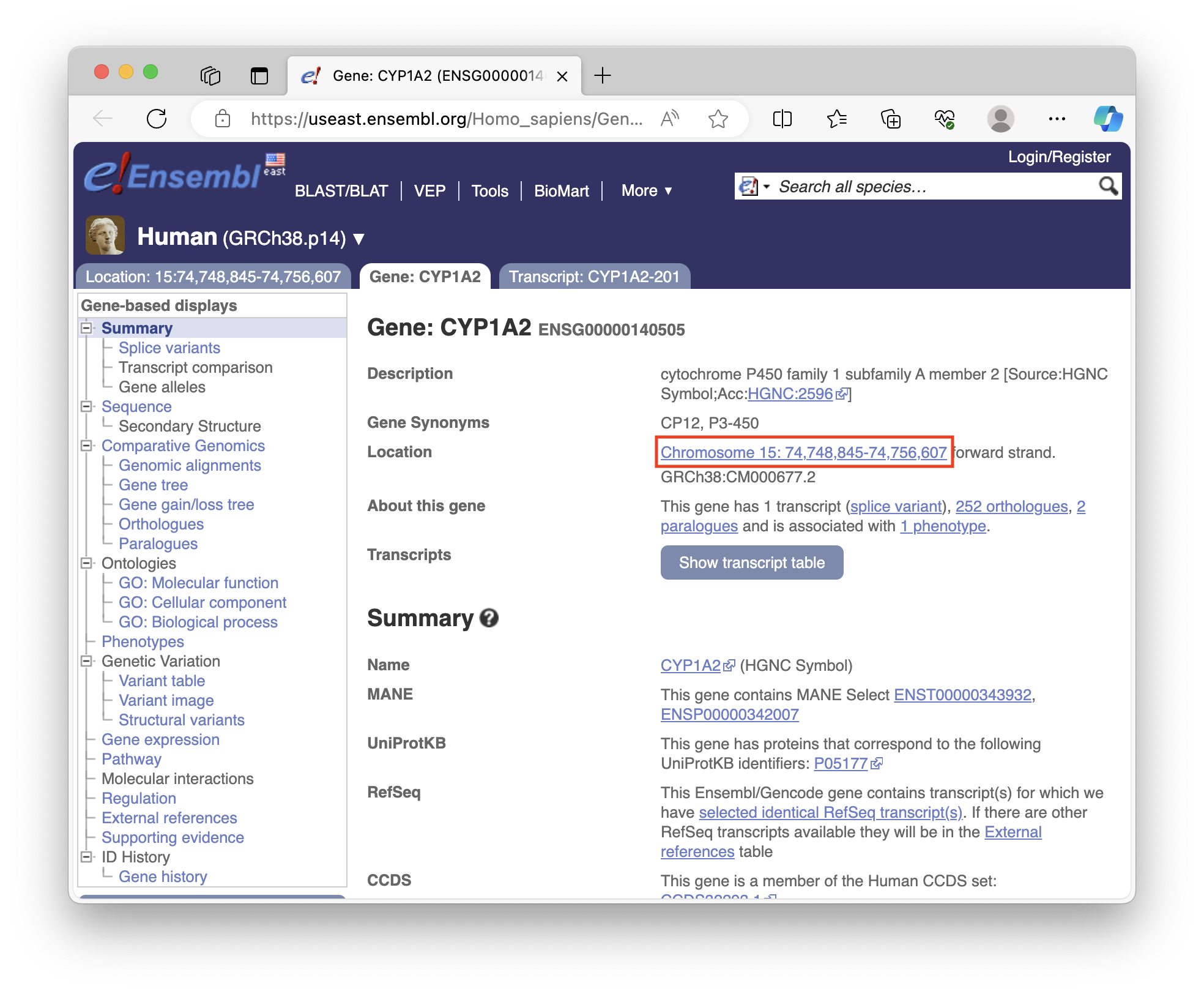
You need to convert the coordinate information into the following format to plot it in IGV notebook:
"chr15:74,748,845-74,756,607", # CYP1A2 coordinates
Paths are relative to the directory in which JupyterLab server was started.
The "tracks" component is where track files are specified after Browser initialization.
Visualize alignment (.bam) and variant call (.vcf) files for to Your Assigned Gene [sname_2]([sid_2])
Lookup locus coordinate information for Your Assigned Gene [sname_2]([sid_2]) using
Ensembl and create another codeblock to visualize
as we did above with the Example Gene [sname_1]([sid_1]):
[sname_2]([sid_2]) on Ensembl and format the like "chr15:74,748,845-74,756,607".igv_notebook to set up visualization. Adjust "genome", "locus", and "tracks" for your gene as we did for Example Gene [sname_1]([sid_1]).zoom_in() for a closer look.minimap2 + clair3 alignment on IGV for Your Assigned Gene [sname_2]([sid_2]) using the button (or take a screenshot). This process mirrors the CYP1A2 example, allowing you to visualize your gene's alignment and variant calls.
Supplementary Information
bedtools sort -i ~/refs/Alliance_PGx_LR_Pnl_TargetsCaptured_hg38_ann.bed | bedtools merge -i - > ~/refs/cleaned_Alliance_PGx_LR_Pnl_TargetsCaptured_hg38_ann.bed
bedtools getfasta -fi ~/refs/Homo_sapiens_assembly38.fasta -bed ~/refs/cleaned_Alliance_PGx_LR_Pnl_TargetsCaptured_hg38_ann.bed -fo ~/refs/cleaned_extracted_regions.fasta
samtools faidx /home/bench-user/refs/cleaned_extracted_regions.fasta
minimap2 -d ~/refs/cleaned_extracted_regions.mmi ~/refs/cleaned_extracted_regions.fasta
Now we'll perform alignment and variant calling on the Oxford Nanopore PGx amplicon data using Clara NVIDIA Parabricks implementation of minimap2 deepvariant.
Step 1: Alignment with minimap2
pbrun minimap2 \
    --ref ~/refs/Homo_sapiens_assembly38.fasta \
    --in-fq ~/ONT_data/fastq/concat_fastq_1000-1025_runid_7c299c5f19bd1502f6745a5c07d438f287c804ab.fastq \
    --out-bam ~/ONT_data/pb_ont_aligned.bam
Step 2: Variant Calling with DeepVariant
pbrun deepvariant \
    --ref ~/refs/Homo_sapiens_assembly38.fasta \
    --in-bam ~/ONT_data/pb_ont_aligned.bam \
    --out-variants ~/ONT_data/pb_variants.vcf \
    --mode ont
Step 3: Visualize the results
Visualize the results for the alignment (.bam) and variant call (.vcf) files for the Example Gene [sname_1]([sid_1]) and Your Assigned Gene [sname_2]([sid_2]).
Add two more cells to your IGV Jupyter notebook abd visualize the first Example Gene [sname_1]([sid_1]) and the second Your Assigned Gene [sname_2]([sid_2]) for the Parabricks deepvariant.
In total, you should end up with four IGV code blocks:
minimap2 + clair3 Example Gene [sname_1]([sid_1])minimap2 + clair3 Your Assigned Gene [sname_2]([sid_2])minimap2 + pbrun deepvariant Example Gene [sname_1]([sid_1])minimap2 + pbrun deepvariant Your Assigned Gene [sname_2]([sid_2])Please answer:
1. What was **Your Assigned Gene**?
2. Upload screenshot of IGV of **Your Assigned Gene** for the `minimap2` + `clair3` result, with the `.bam` and `.vcf` tracks visible.
3. Upload an IGV screenshot of **Your Assigned Gene** for the `minimap2` + `pbrun deepvariant` result, with the `.bam` and `.vcf` tracks visible.
4. How would you figure out how many variants you found using `minimap2` + `clair3`? How about `minimap2` + `pbrun deepvariant`?
5. Was there a noticeable performance upgrade between `minimap2` + `clair3` vs `pbrun minimap2` + `pbrun deepvariant`?
Background
The data in this module comes from a study in the Sequencing Quality Control Phase 2 (SEQC2) Consortium. This study addresses the need for accurate tests in precision oncology that can distinguish true cancer-specific mutations from errors introduced at each step of next-generation sequencing (NGS). The study systematically interrogates somatic mutations in paired tumor–normal cell lines across six different centers to identify factors affecting detection reproducibility and accuracy.
The goal was to evaluate the reproducibility of different sample types with varying input amounts and tumor purity, multiple library construction protocols, and processing with nine bioinformatics pipelines. The study aims to understand how these factors influence variant identification in both whole-genome sequencing (WGS) and whole-exome sequencing (WES).
The study found that read coverage and variant callers significantly affect both WGS and WES reproducibility. However, WES performance is also influenced by insert fragment size, genomic copy content, and the global imbalance score (GIV; G > T/C > A).
Analysis Plan
The samples analyzed in this module are from a human breast ductal carcinoma cell line HCC1395 and its normal control, the B lymphoblast cell line HCC1395BL, established from the same patient. These samples were whole exome sequenced as part of an NGS reference dataset and are used to evaluate the reproducibility and accuracy of cancer mutation detection.
In this tutorial you will be analyzing tumor sample paired with a normal control which were whole exome sequenced as part of NGS reference dataset (Zhao et al., 2021).
The sequencing data was downloaded onto your Deep Origin instance from the European Nucleotide Archive (experiments SRX4728517 and SRX4728518).
Both samples were paired-end sequenced on Illumina platform, resulting in two .fastq read files (i.e. R1 and R2) for each:
Normal sample .fastq file names are WES_LL_N_1_R1_001.fastq.gz and WES_LL_N_1_R2_001.fastq.gz.
Tumor cell line .fastq file names are WES_LL_T_1_R1_001.fastq.gz and WES_LL_T_1_R2_001.fastq.gz.
To avoid waiting hours in real time for the results, we've prepaired smaller subsets of the .fastqfiles which have a mini_ prefix.
.fastq contents
The .fastq file stores reads that the sequencing instrument produced as plain text. In our case it is compressed as gunzip, and can be read using zcat command:
zcat ~/WES_data/fastq/WES_LL_T_1_R1_001.fastq.gz | head -4
This will print out the first read in FASTQ format.
Alignment
.fastq files lack positional information and first have to be aligned to the reference genome using the Burrows-Wheeler Aligner (BWA).
Align the normal sample .fastq:
bwa mem -t 2 -M ~/refs/Homo_sapiens_assembly38.fasta \
                ~/WES_data/fastq/mini_WES_LL_N_1_R1_001.fastq.gz \
                ~/WES_data/fastq/mini_WES_LL_N_1_R2_001.fastq.gz > \
                ~/WES_data/mini_WES_normal.sam
Align the tumor .fastq:
bwa mem -t 2 -M ~/refs/Homo_sapiens_assembly38.fasta \
                ~/WES_data/fastq/mini_WES_LL_T_1_R1_001.fastq.gz \
                ~/WES_data/fastq/mini_WES_LL_T_1_R2_001.fastq.gz > \
                ~/WES_data/mini_WES_tumor.sam
.fasta filebwa outputs into STDOUT by default, so the redirection operator > is used to write to a file.
\ (backslash) character is used to continue a single-line command on the next line.
GATK
All following steps will use tools from the Genome Analysis Toolkit.
Fixing Mate Information
This GATK tool ensures that all mate-pair information is in sync between each read and its mate pair.
This will simultaneously compress text-based .sam (Sequence Alignment Map) file into .bam (Binary Alignment Map).
Control
gatk --java-options "-Xms80G -Xmx480G" FixMateInformation \
                    -I ~/WES_data/mini_WES_normal.sam \
                    -O ~/WES_data/mini_WES_normal.fix.bam \
                    -SO coordinate \
                    -VALIDATION_STRINGENCY SILENT
Tumor
gatk --java-options "-Xms80G -Xmx480G" FixMateInformation \
                    -I ~/WES_data/mini_WES_tumor.sam \
                    -O ~/WES_data/mini_WES_tumor.fix.bam \
                    -SO coordinate \
                    -VALIDATION_STRINGENCY SILENT
.sam file.bam fileAdd Or Replace Read Groups
Write the read group information into .bam. GATK tools need this information to know that certain reads were sequenced together, as they attempt to compensate for variability from one sequencing run to the next.
Control
gatk --java-options "-Xms80G -Xmx480G" AddOrReplaceReadGroups \
        -I ~/WES_data/mini_WES_normal.fix.bam \
        -O ~/WES_data/mini_WES_normal.fix.rg.bam \
        -RGID "SRR7890851" \
        -SM "WES_LL_N_1" \
        -PU "SRR7890851.1" \
        -LB "HS" \
        -PL "ILLUMINA"
Tumor
gatk --java-options "-Xms80G -Xmx480G" AddOrReplaceReadGroups \
        -I ~/WES_data/mini_WES_tumor.fix.bam \
        -O ~/WES_data/mini_WES_tumor.fix.rg.bam \
        -RGID "SRR7890850" \
        -SM "WES_LL_T_1" \
        -PU "SRR7890850.1" \
        -LB "HS" \
        -PL "ILLUMINA"
.bam file.bam fileFor the Illumina-generated files, these values usually mean the following:
Mark duplicate reads
Library preparation includes DNA amplification. The sequences cloned during that step carry the same Unique Molecular Identifier sequence, allowing us to mark the amplified reads to distinguish them from truly identical reads in the sample.
Control
gatk MarkDuplicatesSpark \
        -I ~/WES_data/mini_WES_normal.fix.rg.bam \
        -O ~/WES_data/mini_WES_normal.fix.rg.md.bam \
        -M ~/WES_data/mini_WES_normal.dupl_metrics.txt \
        --conf "spark.executor.cores=2"
gatk MarkDuplicatesSpark \
        -I ~/WES_data/mini_WES_tumor.fix.rg.bam \
        -O ~/WES_data/mini_WES_tumor.fix.rg.md.bam \
        -M ~/WES_data/mini_WES_tumor.dupl_metrics.txt \
        --conf "spark.executor.cores=2"
.bam file
* -O: Output .bam file
* -M: Duplicate mertics output table
* --conf: Spark properties spark.executor.cores specifies number of processor threads.
Create base quality recalibration table
The variant calling relies on probability calculations using quality scores of the read nucleotides. This step attempts to remove noise produced by sequencer's systematic technical errors using an ML algorithm. More on how this works in the GATK documentation.
Create recalibration tables:
Control
gatk BaseRecalibrator \
        -I ~/WES_data/mini_WES_normal.fix.rg.md.bam \
        -R ~/refs/Homo_sapiens_assembly38.fasta \
        --known-sites ~/refs/Homo_sapiens_assembly38.dbsnp138.vcf \
        --known-sites ~/refs/Homo_sapiens_assembly38.known_indels.vcf.gz \
        --known-sites ~/refs/Mills_and_1000G_gold_standard.indels.hg38.vcf.gz \
        -O ~/WES_data/mini_WES_normal.recal_data.table
gatk BaseRecalibrator \
        -I ~/WES_data/mini_WES_tumor.fix.rg.md.bam \
        -R ~/refs/Homo_sapiens_assembly38.fasta \
        --known-sites ~/refs/Homo_sapiens_assembly38.dbsnp138.vcf \
        --known-sites ~/refs/Homo_sapiens_assembly38.known_indels.vcf.gz \
        --known-sites ~/refs/Mills_and_1000G_gold_standard.indels.hg38.vcf.gz \
        -O ~/WES_data/mini_WES_tumor.recal_data.table
.bam fileApply base quality recalibration table
This command applies the recalibration information from the tables to the .bam files.
Control
gatk ApplyBQSR \
        -I ~/WES_data/mini_WES_normal.fix.rg.md.bam \
        -R ~/refs/Homo_sapiens_assembly38.fasta \
        --bqsr-recal-file ~/WES_data/mini_WES_normal.recal_data.table \
        -O ~/WES_data/mini_WES_normal.fix.rg.md.bqsr.bam
gatk ApplyBQSR \
        -I ~/WES_data/mini_WES_tumor.fix.rg.md.bam \
        -R ~/refs/Homo_sapiens_assembly38.fasta \
        --bqsr-recal-file ~/WES_data/mini_WES_tumor.recal_data.table \
        -O ~/WES_data/mini_WES_tumor.fix.rg.md.bqsr.bam
Call somatic variants using Mutect2
After all previous steps are done for both control and tumor samples, we can run variant calling:
gatk Mutect2 --native-pair-hmm-threads 2 \
            -I ~/WES_data/mini_WES_normal.fix.rg.md.bqsr.bam \
            -I ~/WES_data/mini_WES_tumor.fix.rg.md.bqsr.bam \
            --normal WES_LL_N_1 \
            -R ~/refs/Homo_sapiens_assembly38.fasta \
            --germline-resource ~/refs/af-only-gnomad.hg38.vcf.gz \
            -O ~/WES_data/mini_WES_tumor.unfiltered.vcf
SM read group value)
* -R: Reference genome
* --germline-resource: Germline reference .vcf
* -O: Output .vcf
Filter called variants
gatk FilterMutectCalls \
        -R ~/refs/Homo_sapiens_assembly38.fasta \
        -V ~/WES_data/mini_WES_tumor.unfiltered.vcf \
        -O ~/WES_data/mini_WES_tumor.filtered.vcf
Functional annotation
gatk Funcotator \
        --variant ~/WES_data/mini_WES_tumor.filtered.vcf \
        --reference ~/refs/Homo_sapiens_assembly38.fasta \
        --ref-version hg38 \
        --data-sources-path ~/refs/funcotator_dataSources.v1.7.20200521s \
        --output ~/WES_data/mini_WES_tumor.annotated.vcf \
        --output-file-format VCF
NVIDIA Clara Parabricks
Parabricks GPU-accelerated implementation of BWA-GATK4 pipeline can be run using a single command, which combines steps from alignment to Mutect2 variant calling.
pbrun somatic --ref ~/refs/Homo_sapiens_assembly38.fasta \
        --low-memory \
        --in-normal-fq  ~/WES_data/fastq/mini_WES_LL_N_1_R1_001.fastq.gz \
                        ~/WES_data/fastq/mini_WES_LL_N_1_R2_001.fastq.gz \
        --in-tumor-fq   ~/WES_data/fastq/mini_WES_LL_T_1_R1_001.fastq.gz \
                        ~/WES_data/fastq/mini_WES_LL_T_1_R2_001.fastq.gz \
        --fix-mate \
        --normal-read-group-id-prefix "SRR7890851.1" \
        --normal-read-group-sm "WES_LL_N_1" \
        --normal-read-group-lb "HS" \
        --normal-read-group-pl "ILLUMINA" \
        --tumor-read-group-id-prefix "SRR7890850.1" \
        --tumor-read-group-sm "WES_LL_T_1" \
        --tumor-read-group-lb "HS" \
        --tumor-read-group-pl "ILLUMINA" \
        --knownSites ~/refs/Homo_sapiens_assembly38.dbsnp138.vcf \
        --knownSites ~/refs/Homo_sapiens_assembly38.known_indels.vcf.gz \
        --knownSites ~/refs/Mills_and_1000G_gold_standard.indels.hg38.vcf.gz \
        --out-normal-bam ~/WES_data/pb_mini_WES_normal.bam \
        --out-tumor-bam ~/WES_data/pb_mini_WES_tumor.bam \
        --out-normal-recal-file ~/WES_data/pb_mini_WES_normal.recal \
        --out-tumor-recal-file ~/WES_data/pb_mini_WES_tumor.recal \
        --out-vcf ~/WES_data/pb_mini_WES_tumor.unfiltered.vcf
Input files options:
Pipeline steps options:
* --fix-mate: Add mate cigar (MC) and mate quality (MQ) tags to the output file.
* --knownSites: VCF reference for known SNVs. Same as for BaseRecalibrator step of classic BWA-GATK4 pipeline
The following are analogous for AddOrReplaceReadGroups step of classic BWA-GATK4 pipeline:
The rest of the options specify where to store the outputs:
VCF filtering and annotation
Parabricks pipeline does not include VCF filtering and functional annotation steps. We will run these using classic GATK:
Variant quality filtering:
gatk FilterMutectCalls \
        -R ~/refs/Homo_sapiens_assembly38.fasta \
        -V ~/WES_data/pb_mini_WES_tumor.unfiltered.vcf \
        -O ~/WES_data/pb_mini_WES_tumor.filtered.vcf
Functional annotation:
gatk Funcotator \
        --variant ~/WES_data/pb_mini_WES_tumor.filtered.vcf \
        --reference ~/refs/Homo_sapiens_assembly38.fasta \
        --ref-version hg38 \
        --data-sources-path ~/refs/funcotator_dataSources.v1.7.20200521s \
        --output ~/WES_data/pb_mini_WES_tumor.annotated.vcf \
        --output-file-format VCF
Open /WES/Empty_VCF_vizualizations.Rmd in RStudio and build an R Markdown Notebook with these steps:
---
title: "QC and filtering of annotated VCF files"
output: html_notebook
---
Load Libraries
suppressPackageStartupMessages({
  library(VariantAnnotation)
  library(tidyverse)
  library(RColorBrewer)
  library(ggrepel)
  library(cowplot)
})
Load and process VCF files
First, we need to load the VCF files using readVcf function from VariantAnnotation package. We load both classic GATK and Parabricks GATK VCFs as objects into a named list.
vcf.filenames <- c("classic GATK" = "~/WES_data/vcf_analysis/WES_tumor.annotated.vcf",
                   "Parabricks GATK" = "~/WES_data/vcf_analysis/PB_WES_tumor.annotated.vcf")

vcf.list <- lapply(vcf.filenames, readVcf, genome = "hg38")
Here's what looking at dimensions of each element of this list gives us:
lapply(vcf.list, dim)
First value is the number of mutations and the second is the number of samples (normal and tumor). Let's subset the VCF objects leaving only variants which passed the FilterMutectCalls filters:
vcf.list.qc <-
  lapply(vcf.list, function(x)
    x[rowRanges(x)$FILTER == "PASS"])

# Also, filter only variants mapped correctly to a chromosome:
vcf.list.qc <-
  lapply(vcf.list.qc, function(x)
    x[!(grepl(names(x), pattern = "chrUn_")),])

lapply(vcf.list.qc, dim)
Next block of code will extract only the relevant fields and columns from the VCF objects, creating a data frame where each row is a detected variant. It will include positional information and annotations of interest (gene name, type of SNV, allelic frequence) along with additional filter information which we will use to further prune the variants.
extractFUNCOTATION <-
  function(vcf,
           fields = c(
             "Gencode_34_hugoSymbol",
             "Gencode_34_variantClassification",
             "Gencode_34_secondaryVariantClassification",
             "Gencode_34_variantType"
           )) {
    annotation_colnames <-
      info(vcf@metadata$header)["FUNCOTATION", "Description"] %>%
      stringr::str_remove("Functional annotation from the Funcotator tool.  Funcotation fields are: ") %>%
      stringr::str_split(pattern = "\\|") %>%
      unlist()

    as.data.frame(info(vcf)[["FUNCOTATION"]]) %>%
      dplyr::select("FUNCOTATION" = value) %>%
      dplyr::mutate(
        FUNCOTATION = word(FUNCOTATION, 1, sep = "\\]"),
        FUNCOTATION = str_remove_all(FUNCOTATION, "[\\[\\]]")
      ) %>%
      tidyr::separate(FUNCOTATION,
                      into = annotation_colnames,
                      sep = "\\|",
                      fill = "right") %>%
      dplyr::select(all_of(fields))
  }

vcf.list.anno <- lapply(vcf.list.qc, function(x) extractFUNCOTATION(x))

snv.list <- list()
for(sample.name in names(vcf.list.qc)) {
  vcf <- vcf.list.qc[[sample.name]]
  df.anno <- vcf.list.anno[[sample.name]]
  snv.list[[sample.name]] <- as.data.frame(geno(vcf)[["AF"]]) %>%

    # since the sample is the same in both VCF, we rename the AF columns equally
    setNames(., c("AF_CTRL", "AF_TUMOR")) %>%

    mutate_all( ~ unlist(.)) %>%
    cbind(., df.anno) %>%
    mutate(
      DP = info(vcf)[["DP"]],
      TLOD = info(vcf)[["TLOD"]] %>% unlist()
    ) %>%
    rownames_to_column("Variant") %>%
    mutate(Position_hg38 = word(Variant, 1, sep = "_"),
           .before = "Variant") %>%
    mutate(Variant = word(Variant, 2, sep = "_"))
}

lapply(snv.list, head, 10) # Print only first 10 rows
Variant filters
Most of these SNVs are artefacts that we will need to filter out.
First, we can remove non-coding variants: introns, variants from intergenic regions, etc. Next block of code creates a second_filter column in the data frame with SNVs which will help us filter the mutations without losing possible false negatives.
noncoding.vars <- c("IGR", "INTRON", "COULD_NOT_DETERMINE", "RNA", "SILENT")

snv.list <- snv.list %>%
  lapply(
  mutate,
    second_filter = case_when(
      Gencode_34_variantClassification %in% noncoding.vars ~ "non-coding",
      Gencode_34_secondaryVariantClassification %in% noncoding.vars ~ "non-coding",
      TRUE ~ "PASS"
    )
  )

lapply(snv.list, filter, second_filter == "PASS") %>%
  lapply(dim)
Next, we can filter the mutations by thresholding them by tumor allele frequency > 10% and TLOD > 15. TLOD stands for tumor log odds and is a of probability that the variant is present in the tumor sample relative to the expected noise.
AF_TUMOR_thresh <- 0.1
TLOD_thresh <- 15

snv.list <- snv.list %>%
  lapply(
    mutate,
    second_filter = case_when(
      second_filter == "PASS" & TLOD < TLOD_thresh ~ "low_TLOD",
      second_filter == "PASS" &
        AF_TUMOR < AF_TUMOR_thresh ~ "low_TUMOR_AF",
      TRUE ~ second_filter
    )
  )

lapply(snv.list, filter, second_filter == "PASS") %>%
  lapply(dim)
The above chunk also outputs the number of SNVs left after filtering out con-coding variants.
max.TLOD <- bind_rows(snv.list) %>%
  select(TLOD) %>% max()
min.TLOD <- bind_rows(snv.list) %>%
  select(TLOD) %>% min()

lapply(names(snv.list),
       function(name) {
         snv.list[[name]] %>%
           filter(second_filter != "non-coding") %>%
           ggplot(aes(y = AF_TUMOR, x = TLOD)) +
           theme_bw() +
           labs(title = name) +
           geom_point(
             aes(color = Gencode_34_variantClassification),
             shape = 1,
             size = 2,
             stroke = 1
           ) +
           scale_y_continuous(labels = scales::percent, limits = c(0, 1)) +
           scale_x_continuous(
             trans = "log10",
             limits = c(min.TLOD, max.TLOD),
             breaks = c(1, 10, 20, 50, 100, 200)
           ) +
           geom_vline(xintercept = TLOD_thresh, linetype = 2) +
           geom_hline(yintercept = AF_TUMOR_thresh, linetype = 2)
       })
This scatterplot shows all coding mutations colored by type. On the X axis is TLOD and allele frequency is on the Y axis. Dotted lines show our thresholds - only mutations in the upper right quadrant will be considered in the downstream analysis.
Compare the allele frequencies for SNV detected in both samples
Let's combine the snv.list into one dataframe and inspect the overlap of filtered mutations:
combined.snv.df <- snv.list %>%
  bind_rows(.id = "pipeline") %>%
  filter(second_filter == "PASS") %>%
  dplyr::select(pipeline, Position_hg38, Variant, AF_TUMOR,
         Gencode_34_hugoSymbol, Gencode_34_variantClassification) %>%
  pivot_wider(names_from = "pipeline", values_from = "AF_TUMOR")

combined.snv.df %>%
  mutate(detection = case_when(
    !is.na(`classic GATK`) & !is.na(`Parabricks GATK`) ~ "classic and Parabricks",
    !is.na(`classic GATK`) & is.na(`Parabricks GATK`) ~ "classic",
    is.na(`classic GATK`) & !is.na(`Parabricks GATK`) ~ "Parabricks"
  )) %>%
  group_by(detection, Gencode_34_variantClassification) %>%
  summarise(N = n()) %>%
  pivot_wider(names_from = detection, values_from = N)
One of the most commonly mutated genes in tumors is TP53. Using filter by gene name we can check the presence of TP53 mutations.
filter(combined.snv.df, Gencode_34_hugoSymbol == "TP53")
Finally, lets compare the allele frequencies for the variants detected by both pipelines:
combined.snv.df %>%
  ggplot(aes(x = `classic GATK`, y = `Parabricks GATK`)) +
  geom_point(aes(fill = Gencode_34_variantClassification),
             shape = 21,
             size = 2) +
  theme_bw() +
  scale_y_continuous(labels = scales::percent, limits = c(0, 1)) +
  scale_x_continuous(labels = scales::percent, limits = c(0, 1))
Session info
sessionInfo()
Your final notebook should look like this.
1. Why is it neccessary to have a Normal sample when performing variant calling?
2. If you have two samples from the same patient and one of them has a significantly lower allele frequency——but the SNV profile is the same——what could the reason for that be?
3. Are their other paramaters or experimental features than can impact variant calling?
File tree:
~/BENCH-USER
├─ MICROBIAL_data/
│  ├─ fastq/
      ├─ JC-0117_S1047_L001_R1_001.fastq.gz
      ├─ JC-0117_S1047_L001_R2_001.fastq.gz
   ├─ microbial_IGV_viz.ipynb
   ├─ GATK_Microbial_calling_local_pjb_new.sh
   ├─ GCF_002890725.1_ASM289072v1_genomic.fa
   ├─ JC-0117.unshifted.vcf
   ├─ JC-0117.unshifted.vcf.idx
   ├─ JC-0117.unshifted.vcf.stats

├─ ONT_data/
│  ├─ fastq/
      ├─ concat_fastq_1000-1025_runid_7c299c5f19bd1502f6745a5c07d438f287c804ab.fastq
      ├─ fastq_runid_7c299c5f19bd1502f6745a5c07d438f287c804ab_1000_0.fastq
      ├─ fastq_runid_7c299c5f19bd1502f6745a5c07d438f287c804ab_1001_0.fastq
      ├─ fastq_runid_7c299c5f19bd1502f6745a5c07d438f287c804ab_1002_0.fastq
      ├─ fastq_runid_7c299c5f19bd1502f6745a5c07d438f287c804ab_1003_0.fastq
      ├─ fastq_runid_7c299c5f19bd1502f6745a5c07d438f287c804ab_1004_0.fastq
      ├─ fastq_runid_7c299c5f19bd1502f6745a5c07d438f287c804ab_1005_0.fastq
      ├─ fastq_runid_7c299c5f19bd1502f6745a5c07d438f287c804ab_1006_0.fastq
      ├─ fastq_runid_7c299c5f19bd1502f6745a5c07d438f287c804ab_1007_0.fastq
      ├─ fastq_runid_7c299c5f19bd1502f6745a5c07d438f287c804ab_1008_0.fastq
      ├─ fastq_runid_7c299c5f19bd1502f6745a5c07d438f287c804ab_1009_0.fastq
      ├─ fastq_runid_7c299c5f19bd1502f6745a5c07d438f287c804ab_1010_0.fastq
      ├─ fastq_runid_7c299c5f19bd1502f6745a5c07d438f287c804ab_1011_0.fastq
      ├─ fastq_runid_7c299c5f19bd1502f6745a5c07d438f287c804ab_1012_0.fastq
      ├─ fastq_runid_7c299c5f19bd1502f6745a5c07d438f287c804ab_1013_0.fastq
      ├─ fastq_runid_7c299c5f19bd1502f6745a5c07d438f287c804ab_1014_0.fastq
      ├─ fastq_runid_7c299c5f19bd1502f6745a5c07d438f287c804ab_1015_0.fastq
      ├─ fastq_runid_7c299c5f19bd1502f6745a5c07d438f287c804ab_1016_0.fastq
      ├─ fastq_runid_7c299c5f19bd1502f6745a5c07d438f287c804ab_1017_0.fastq
      ├─ fastq_runid_7c299c5f19bd1502f6745a5c07d438f287c804ab_1018_0.fastq
      ├─ fastq_runid_7c299c5f19bd1502f6745a5c07d438f287c804ab_1019_0.fastq
      ├─ fastq_runid_7c299c5f19bd1502f6745a5c07d438f287c804ab_1020_0.fastq
      ├─ fastq_runid_7c299c5f19bd1502f6745a5c07d438f287c804ab_1021_0.fastq
      ├─ fastq_runid_7c299c5f19bd1502f6745a5c07d438f287c804ab_1022_0.fastq
      ├─ fastq_runid_7c299c5f19bd1502f6745a5c07d438f287c804ab_1023_0.fastq
      ├─ fastq_runid_7c299c5f19bd1502f6745a5c07d438f287c804ab_1024_0.fastq
      └─ fastq_runid_7c299c5f19bd1502f6745a5c07d438f287c804ab_1025_0.fastq


├─ WES_data/
│  ├─ fastq/
│  │  ├─ mini_WES_LL_T_1_R1_001.fastq.gz
│  │  ├─ mini_WES_LL_T_1_R2_001.fastq.gz
│  │  ├─ mini_WES_LL_N_1_R1_001.fastq.gz
│  │  ├─ mini_WES_LL_N_1_R2_001.fastq.gz
│  ├─ vcf_analysis/
│  │  ├─ WES_tumor.annotated.vcf
│  │  ├─ pb_WES_tumor.annotated.vcf
│  │  ├─ VCF_vizualizations.Rmd
│  │  ├─ VCF_vizualizations.nb.html
│  ├─ exome_IGV_viz.ipynb